5.9 Visualization
5.9.1 Features and annatation data
Several generic functions are available to visualize feature and annotation data:
| Generic | Classes | Remarks |
|---|---|---|
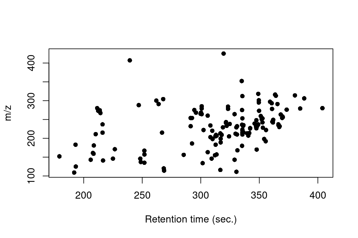
plot() |
featureGroups, featureGroupsComparison |
Scatter plot for retention and m/z values |
plotInt() |
featureGroups |
Intensity profiles across analyses |
plotChroms() |
featureGroups, components |
Plot extracted ion chromatograms (EICs) |
plotSpectrum() |
MSPeakLists, formulas, compounds, components |
Plots (annotated) spectra |
plotStructure() |
compounds |
Draws candidate structures |
plotScores() |
formulas, compounds |
Barplot with candidate scoring |
plot() |
componentsClust |
Creates a dendrogram for the clustered components |
plotGraph() |
componentsNT |
Draws interactive graphs of linked homologous series |
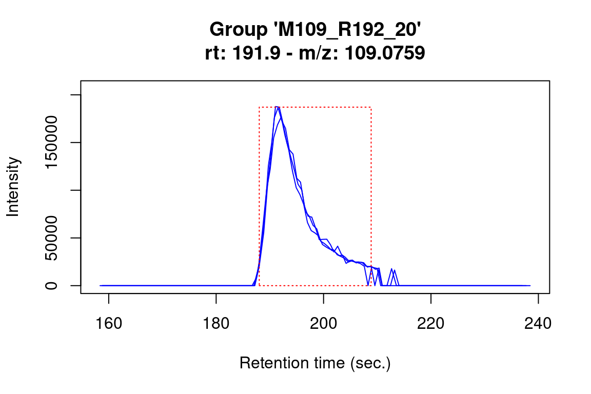
The most common plotting functions are plotChroms(), which plots chromatographic data for features, and plotSpectrum(), which will plot (annotated) spectra. An overview of their most important function arguments are shown below.
| Argument | Generic | Remarks |
|---|---|---|
retMin |
plotChroms() |
If TRUE plot retention times in minutes |
EICParams |
plotChroms() |
Advanced parameters to control the creation of extracted ion chromatograms (described below) |
showPeakArea, showFGroupRect |
plotChroms() |
Fill peak areas / draw rectangles around feature groups? |
title |
plotChroms(), plotSpectrum() |
Override plot title |
showLegend |
plot(), plotInt(), plotChroms() |
Display a legend? |
xlim, ylim |
plotChroms(), plotSpectrum() |
Override x/y axis ranges, i.e. to manually set plotting range. |
groupBy |
plot(), plotInt(), plotChroms() |
Defines if and how data is grouped in the plot (e.g. by replicate) |
groupName, analysis, precursor, index |
plotSpectrum() |
What to plot. See examples below. |
MSLevel |
plotSpectrum() |
Whether to plot an MS or MS/MS spectrum (only MSPeakLists) |
formulas |
plotSpectrum() |
Whether formula annotations should be added (only compounds) |
plotStruct |
plotSpectrum() |
Whether the structure should be added to the plot (only compounds) |
mincex |
plotSpectrum() |
Minimum annotation font size (only formulas/compounds) |
Note that we can use subsetting to select which feature data we want to plot, e.g.
#> Using 'mzr' backend for reading MS data.
#> ================================================================================
#> Using 'mzr' backend for reading MS data.
#> ================================================================================
The plotStructure() function will draw a chemical structure for a compound candidate. In addition, this function can draw the maximum common substructure (MCS) of multiple candidates in order to assess common structural features.
# structure for first candidate
plotStructure(compounds, index = 1, groupName = "M120_R268_30")
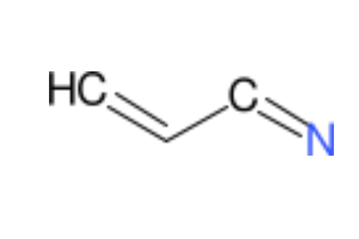
# MCS for first three candidates
plotStructure(compounds, index = 1:3, groupName = "M120_R268_30")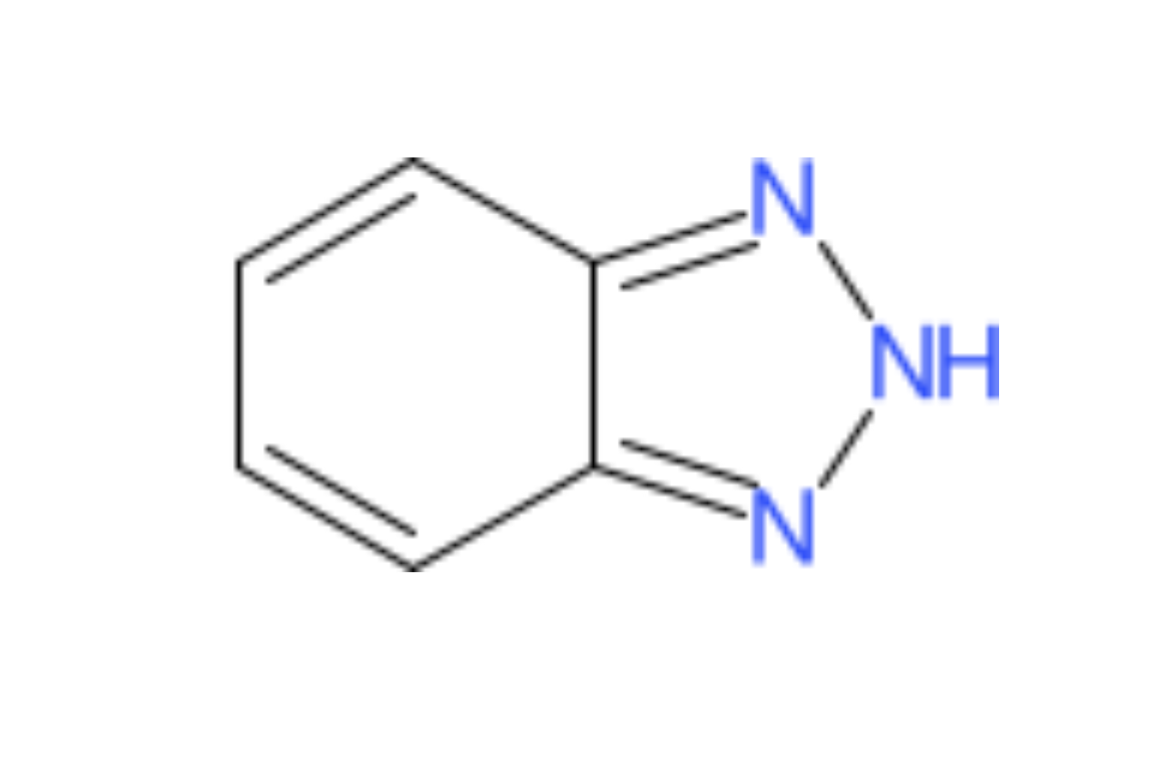
Some other common and less common plotting operations are shown below.
plotInt(fGroups[, 1:10], groupBy = "fGroups") # plot intensities of first ten feature groups and group them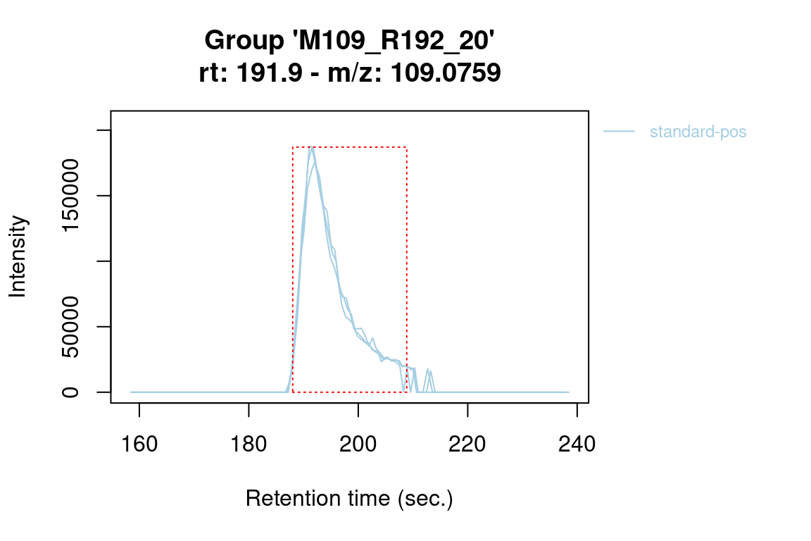
#> Using 'mzr' backend for reading MS data.
#> ================================================================================
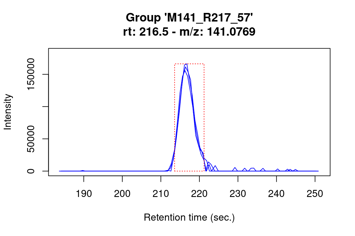
plotChroms(fGroups[, 1], # only plot all features of first group
           groupBy = "replicate") # and mark them individually per replicate
#> Using 'mzr' backend for reading MS data.
#> ================================================================================
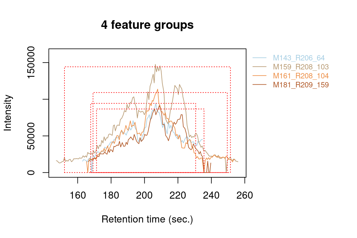
plotChroms(fGroups[, 1:10], # only first ten feature groups
groupBy = "fGroups", # group each feature group
showPeakArea = TRUE, # show integrated areas
showFGroupRect = FALSE) # no rectangles around feature groups#> Using 'mzr' backend for reading MS data.
#> ================================================================================
#> Using 'mzr' backend for reading MS data.
#> ================================================================================
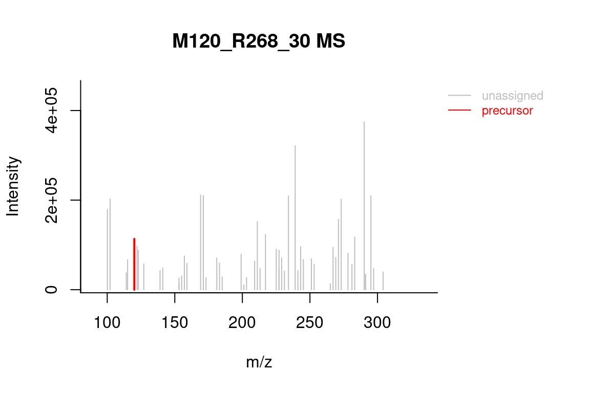
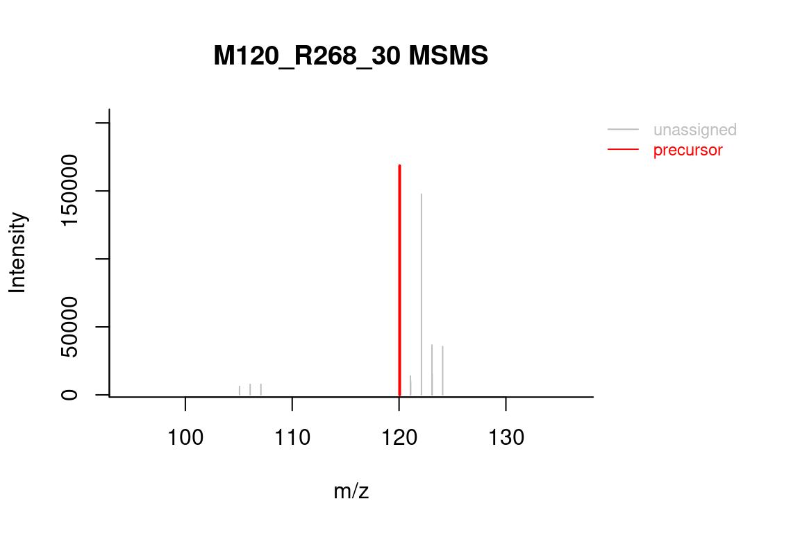
# formula annotated spectrum
plotSpectrum(formulas, index = 1, groupName = "M120_R268_30",
             MSPeakLists = mslists)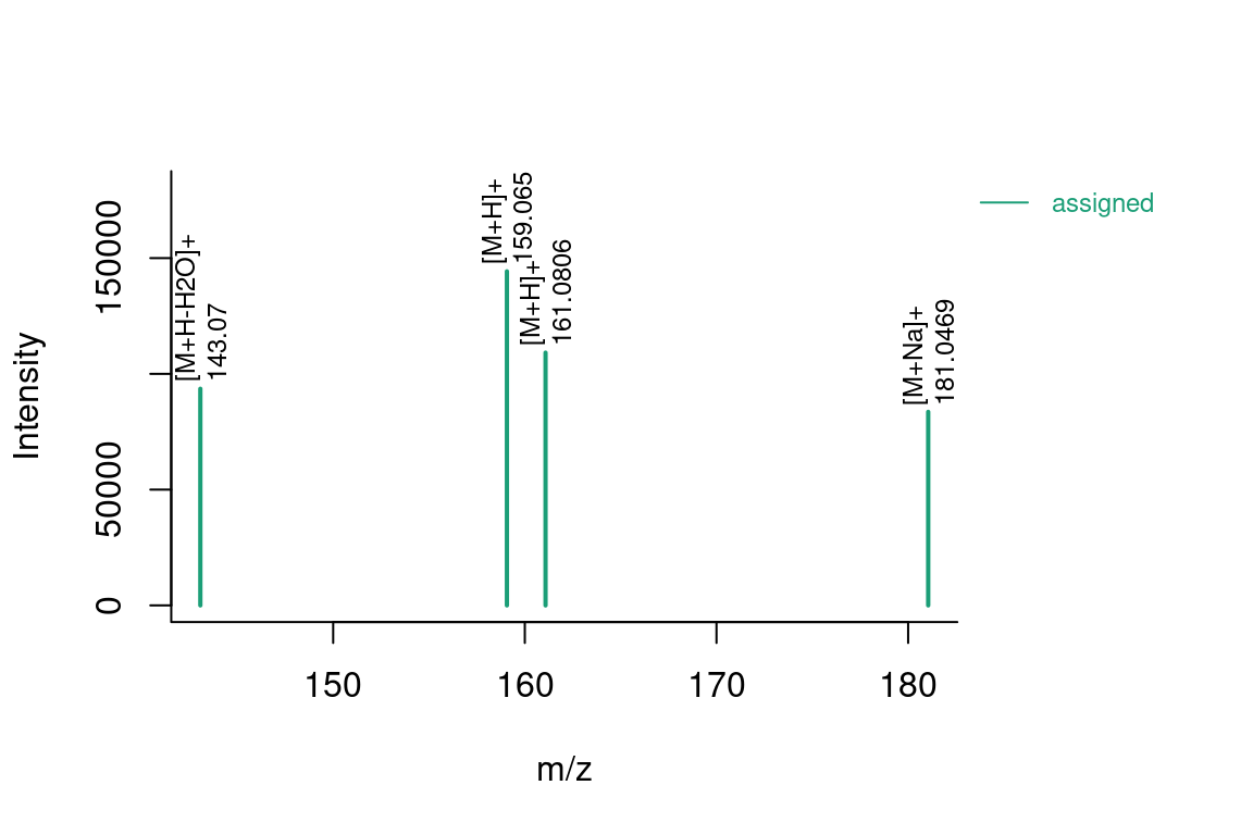
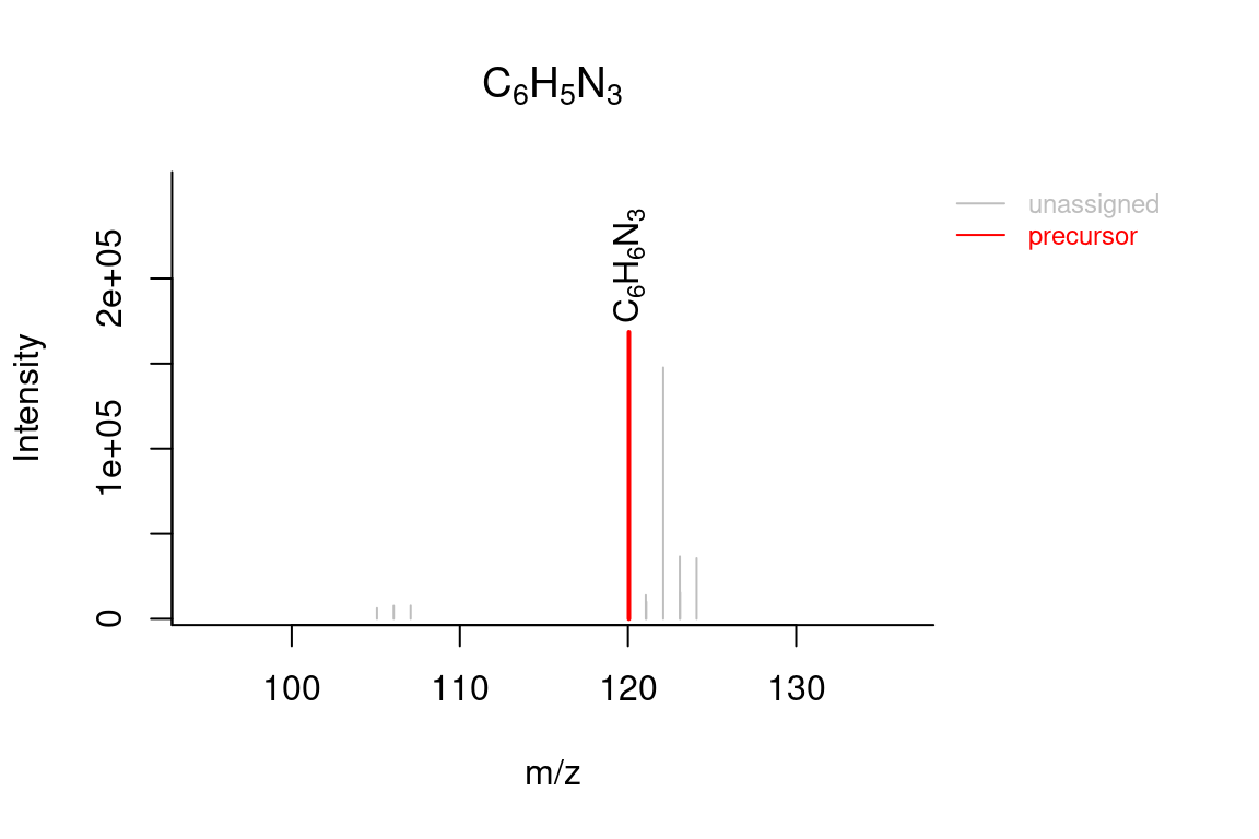
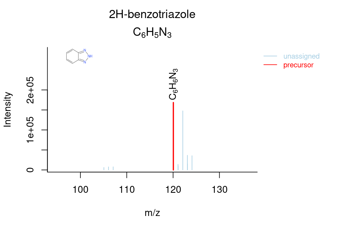
# compound annotated spectrum, with added formula annotations
plotSpectrum(compounds, index = 1, groupName = "M120_R268_30", MSPeakLists = mslists,
             formulas = formulas, plotStruct = TRUE)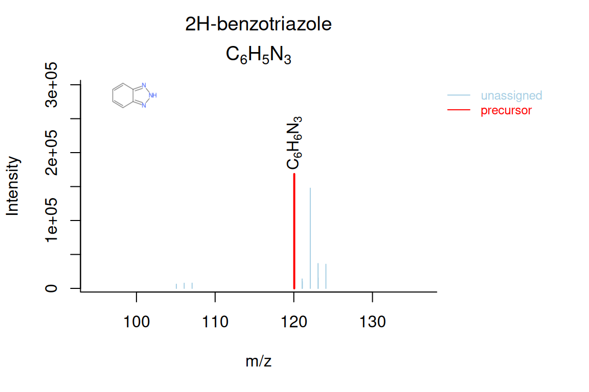
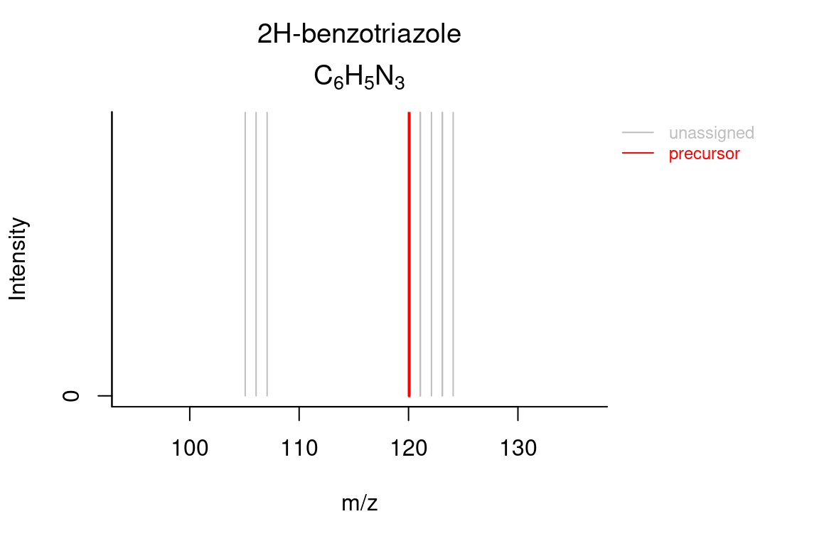
# custom intensity range (e.g. to zoom in)
plotSpectrum(compounds, index = 1, groupName = "M120_R268_30", MSPeakLists = mslists,
             ylim = c(0, 5000), plotStruct = FALSE)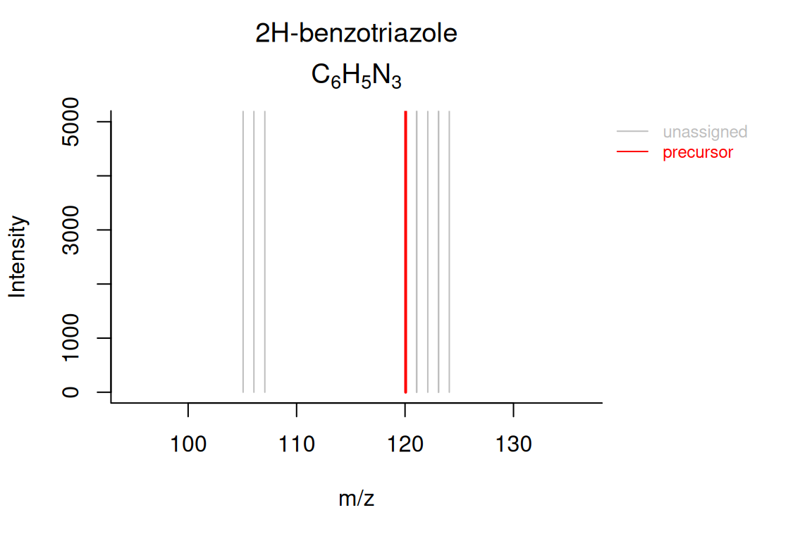

5.9.1.1 Extracted Ion Chromatogram parameters
The EICParams argument to plotChroms() is used to specify more advanced parameters for the creation of extracted ion chromatograms (EICs). Some parameters of interest:
| Parameter | Description |
|---|---|
window |
Expands the EIC retention time range +/- the feature peak width (in seconds). This is e.g. useful to zoom out. |
topMost |
Only consider this amount of highest intensity features in a group. |
topMostByReplicate |
If TRUE then the topMost parameter concerns the top most intense features in a replicate (e.g. topMost=1 would draw the most intense feature for each replicate). |
onlyPresent |
Only create EICs for analyses where a feature was detected? Setting to FALSE is useful to inspect if a feature was ‘missed’. |
The parameters are configured by giving a named list to the EICParams argument. To obtain such a list with default settings, the getDefEICParams() function can be used:
#> $topMost
#> NULL
#>
#> $topMostByReplicate
#> [1] FALSE
#>
#> $onlyPresent
#> [1] TRUE
#>
#> $mzExpWindow
#> [1] 0.001
#>
#> $mobExpWindow
#> [1] 0.01
#>
#> $mzExpMobWindow
#> [1] 0.005
#>
#> $minIntensityIMS
#> [1] 25
#>
#> $setsAdductPos
#> [1] "[M+H]+"
#>
#> $setsAdductNeg
#> [1] "[M-H]-"
#>
#> $window
#> [1] 30
#>
#> $gapFactor
#> [1] 3
Any arguments specified to this function will alter the values of the returned parameter list. Some examples:
# investigate if any features were not detected in a feature group
plotChroms(fGroups[, 10], EICParams = getDefEICParams(onlyPresent = FALSE))
#> Using 'mzr' backend for reading MS data.
#> ================================================================================
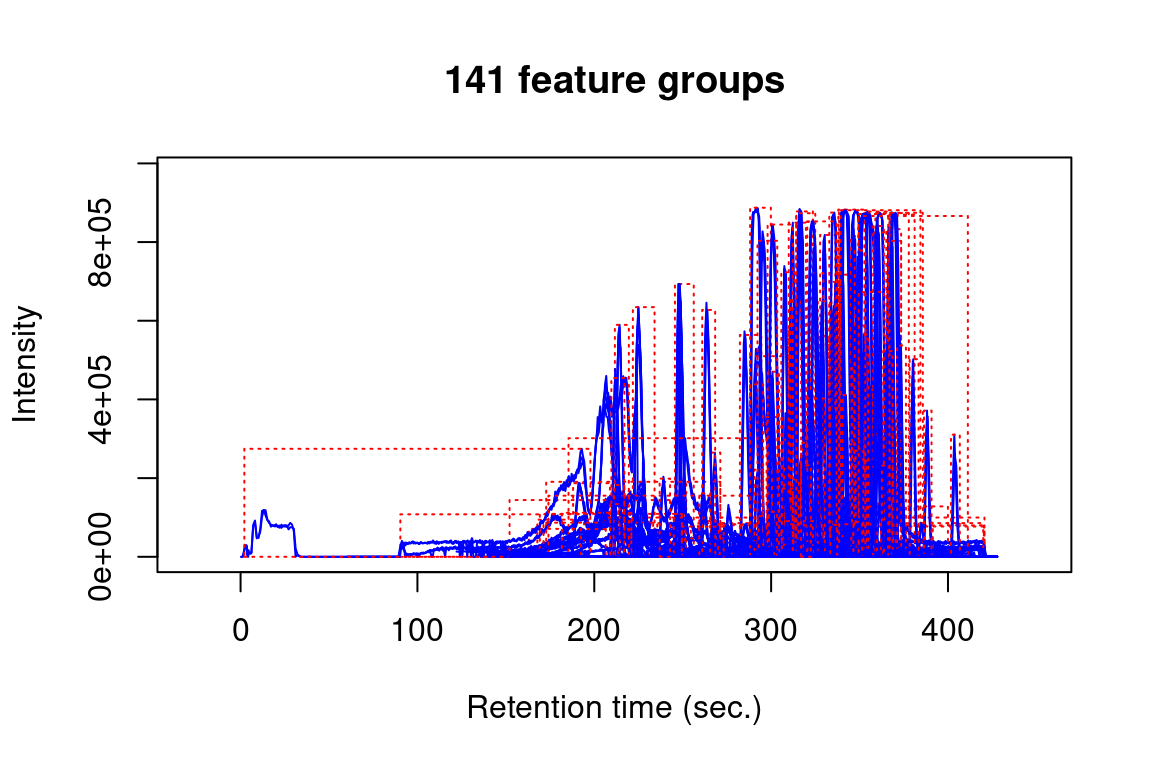
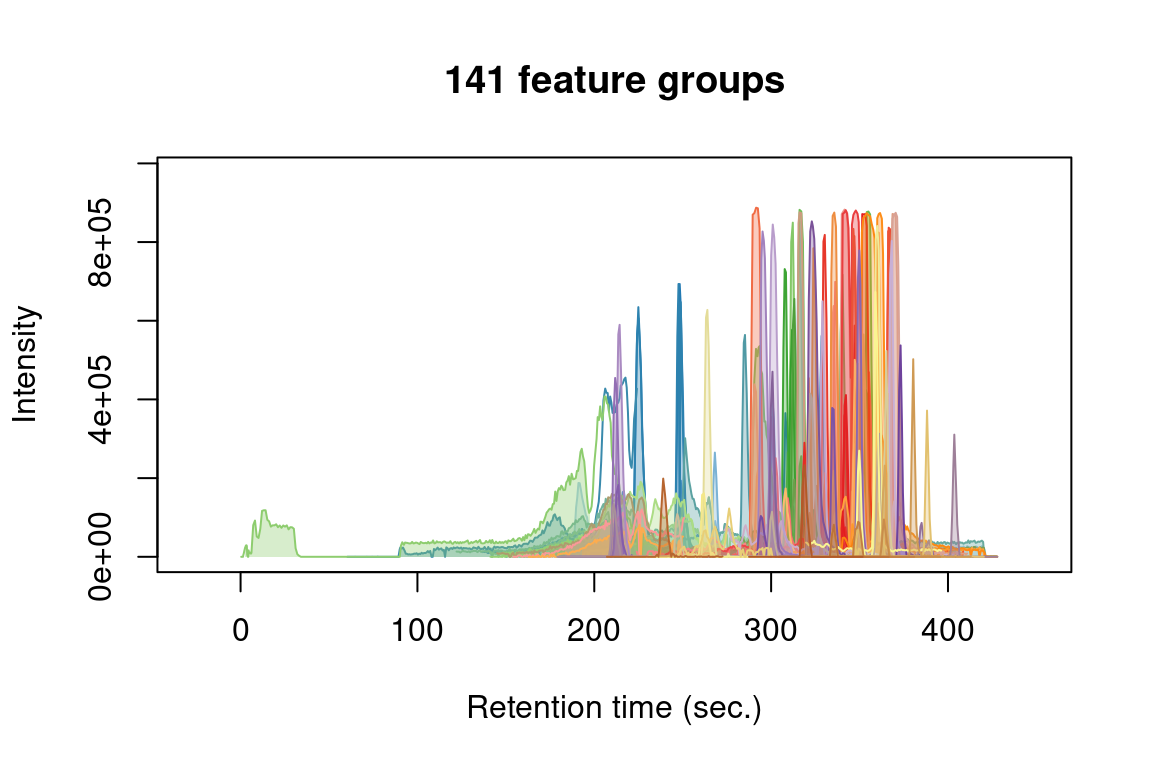
# get overview of all feature groups
plotChroms(fGroups,
           groupBy = "fGroups", # unique colour for each group
           EICParams = getDefEICParams(topMost = 1), # only most intense feature in each group
           showPeakArea = TRUE, # show integrated areas
           showFGroupRect = FALSE,
           showLegend = FALSE) # no legend (too busy for many feature groups)
#> Using 'mzr' backend for reading MS data.
#> ================================================================================
The reference manual (?EICParams) gives a full detail on all parameters.
5.9.2 Overlapping and unique data
There are three functions that can be used to visualize overlap and uniqueness between data:
| Generic | Classes |
|---|---|
plotVenn |
featureGroups, featureGroupsComparison, formulas, compounds |
plotUpSet |
featureGroups, featureGroupsComparison, formulas, compounds |
plotChord |
featureGroups, featureGroupsComparison |
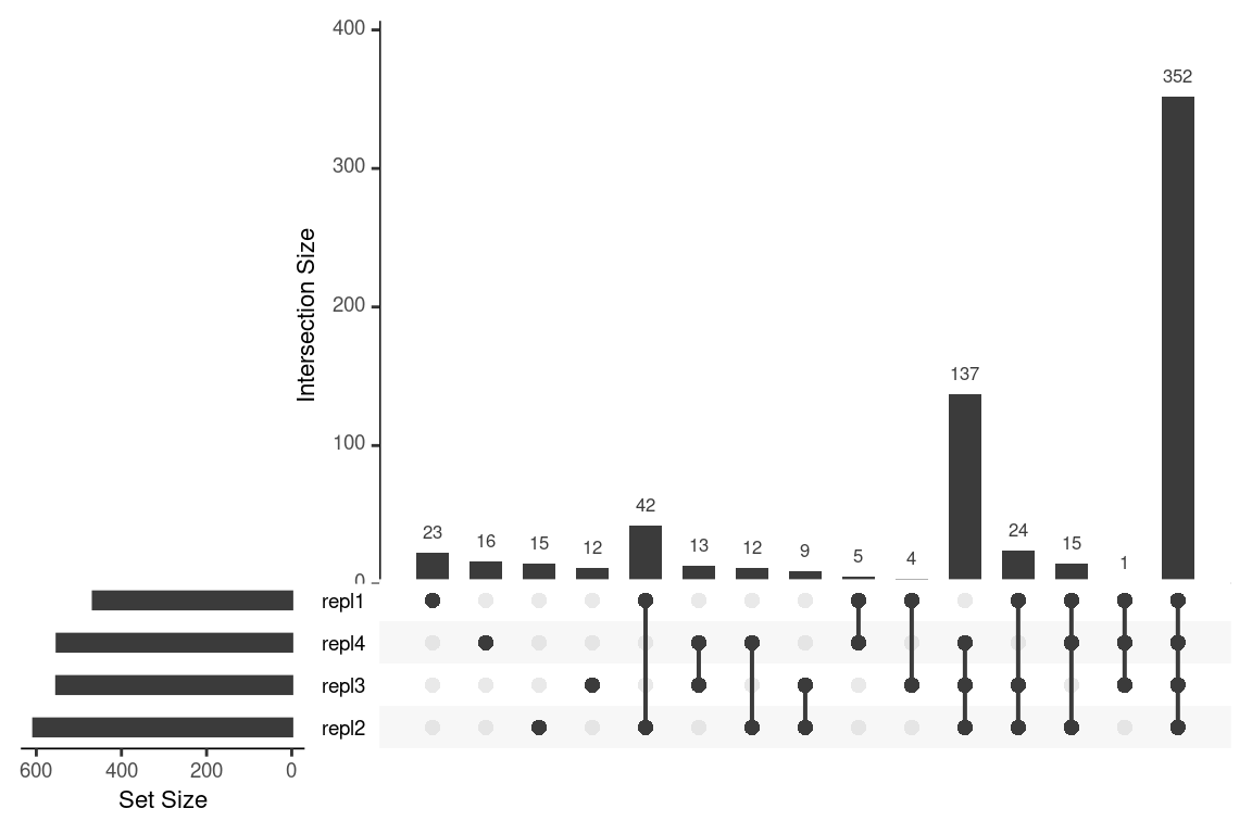
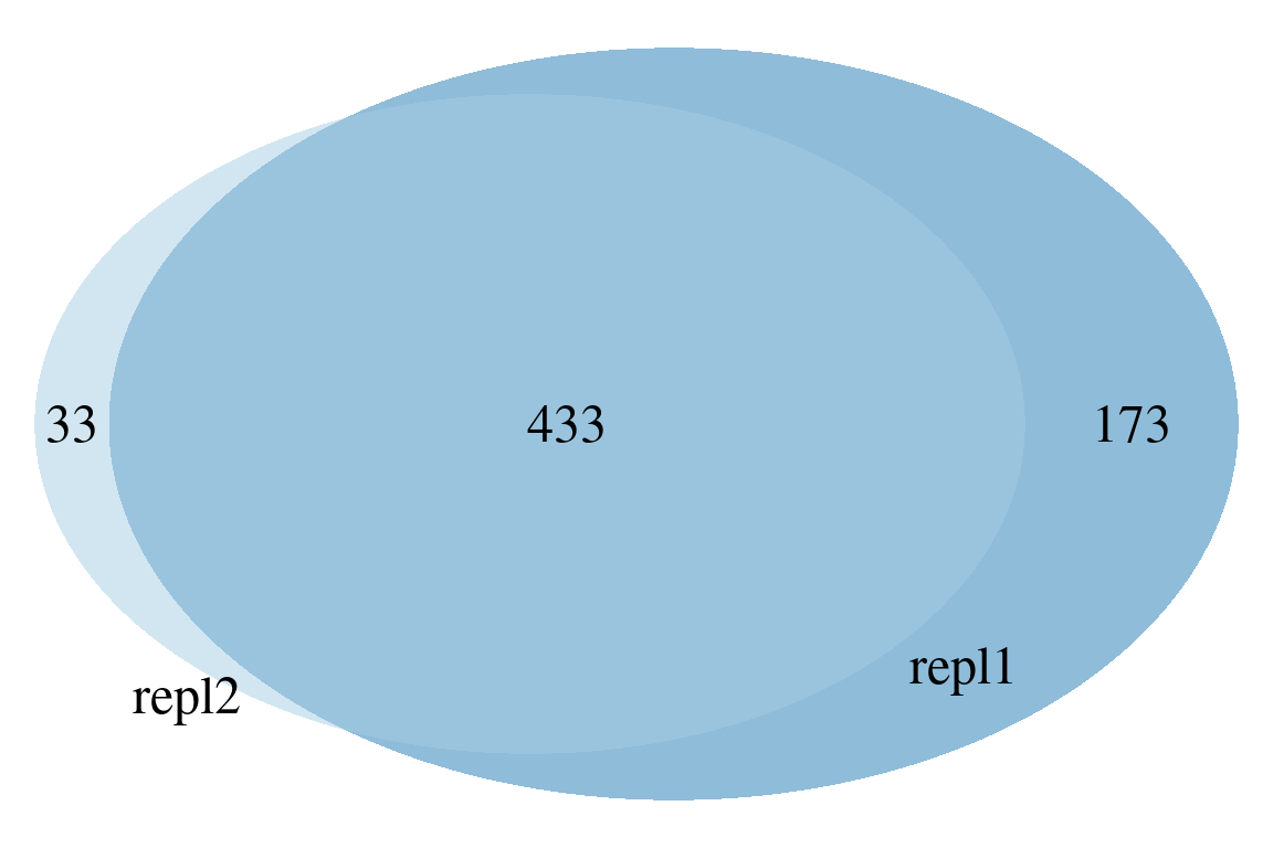
The most simple comparison plot is a Venn diagram (i.e. plotVenn()). This function is especially useful for two or three-way comparisons. More complex comparisons are better visualized with UpSet diagrams (i.e. plotUpSet()). Finally, chord diagrams (i.e. plotChord()) provide visually pleasing diagrams to assess overlap between data.
These functions can either be used to compare feature data or different objects of the same type. The former is typically used to compare overlap or uniqueness between features in different replicates, whereas comparison between objects is useful to visualize differences in algorithmic output. Besides visualization, note that both operations can also be performed to modify or combine objects (see unique and overlapping features and algorithm consensus).
As usual, some examples are shown below.
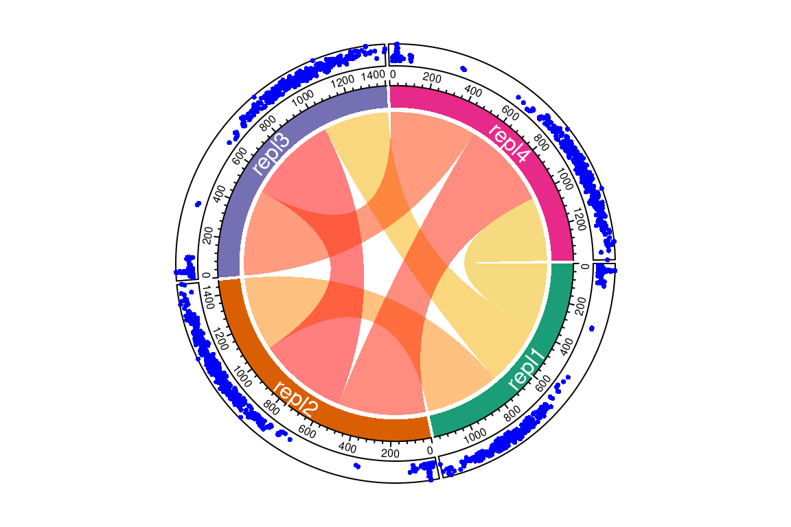
# compare with custom made groups
# plotChord(fGroups, aggregate = TRUE,
#           outer = c(repl1 = "grp1", repl2 = "grp1", repl3 = "grp2", repl4 = "grp3"))

# compare GenForm and SIRIUS results
plotVenn(formsGF, formsSIR,
         labels = c("GF", "SIR")) # manual labeling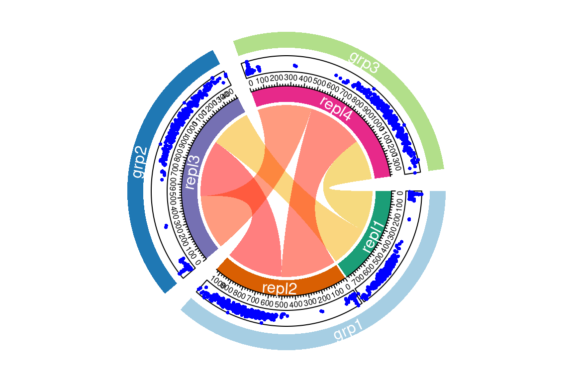
5.9.3 MS similarity
The plotSpectrum function is also useful to visually compare (annotated) spectra. This works for MSPeakLists, formulas and compounds object data.
plotSpectrum(compounds, groupName = c("M120_R268_30", "M146_R309_68"), index = c(1, 1),
             MSPeakLists = mslists)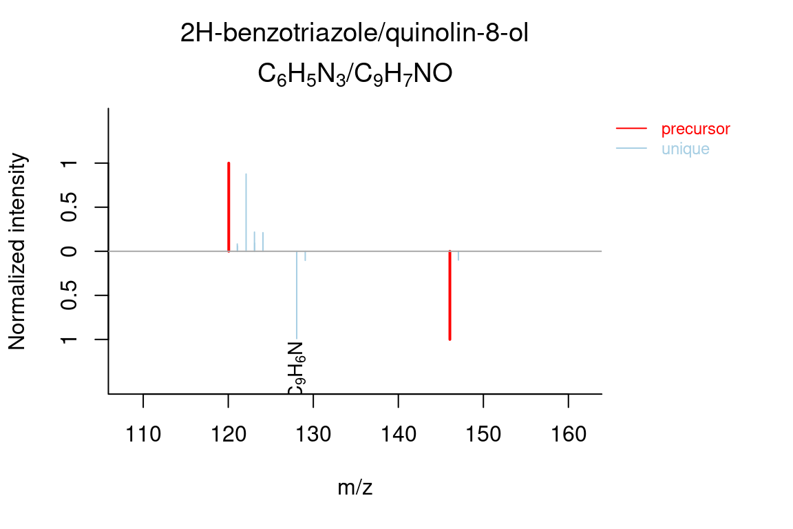
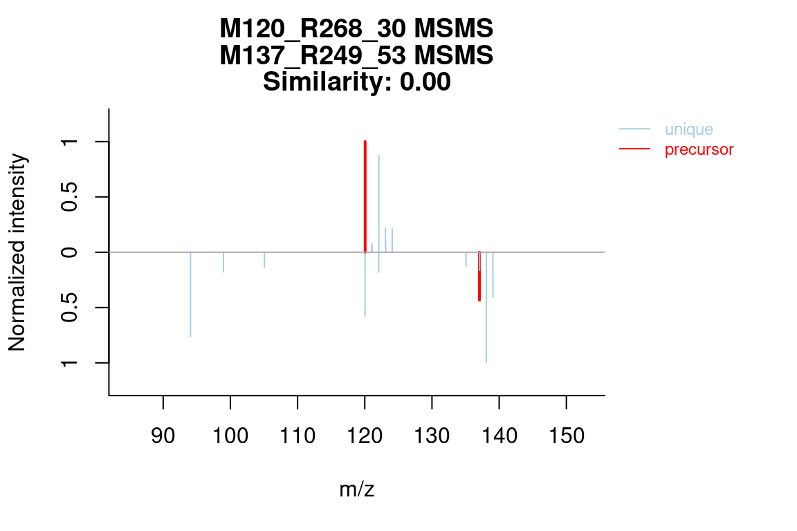
The specSimParams argument, which was discussed in MS similarity, can be used to configure the similarity calculation:
plotSpectrum(mslists, groupName = c("M120_R268_30", "M137_R249_53"), MSLevel = 2,
             specSimParams = getDefSpecSimParams(shift = "both"))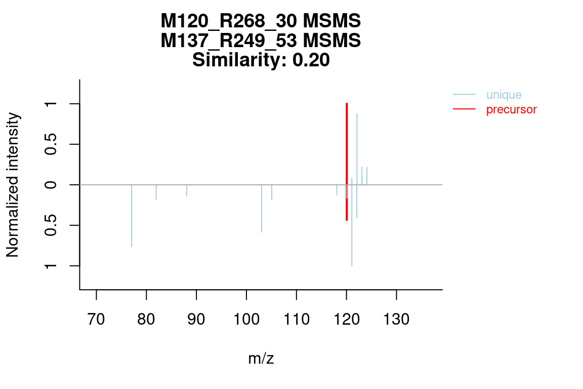
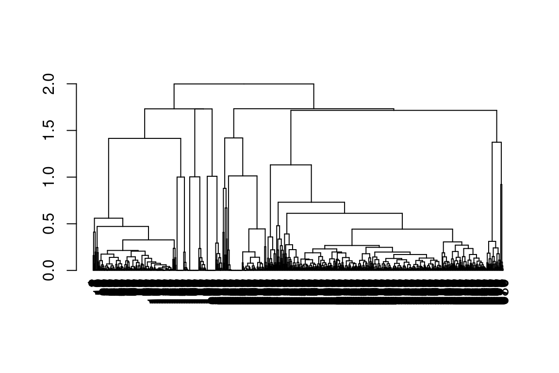
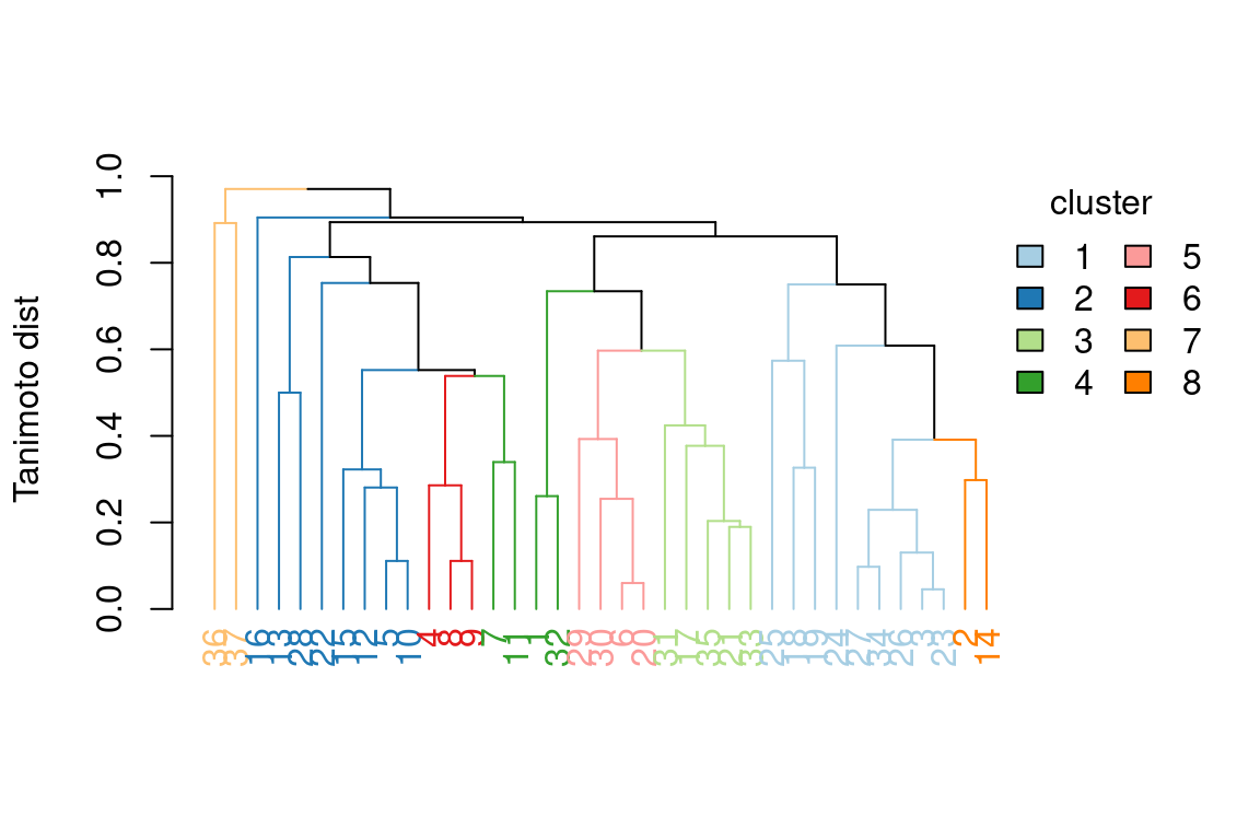
5.9.4 Hierarchical clustering results
In patRoon hierarchical clustering is used for some componentization algorithms and to cluster candidate compounds with similar chemical structure (see compound clustering). The functions below can be used to visualize their results.
| Generic | Classes | Remarks |
|---|---|---|
plot() |
All | Plots a dendrogram |
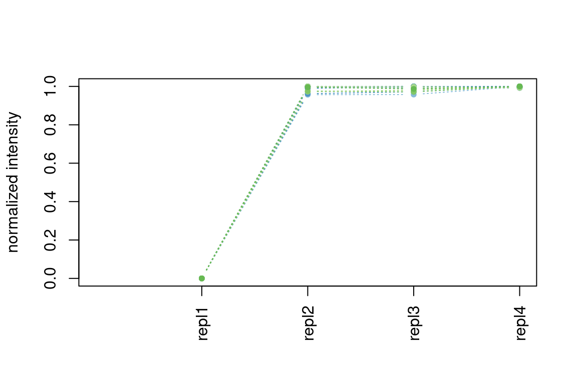
plotInt() |
componentsIntClust |
Plots normalized intensity profiles in a cluster |
plotHeatMap() |
componentsIntClust |
Plots an heatmap |
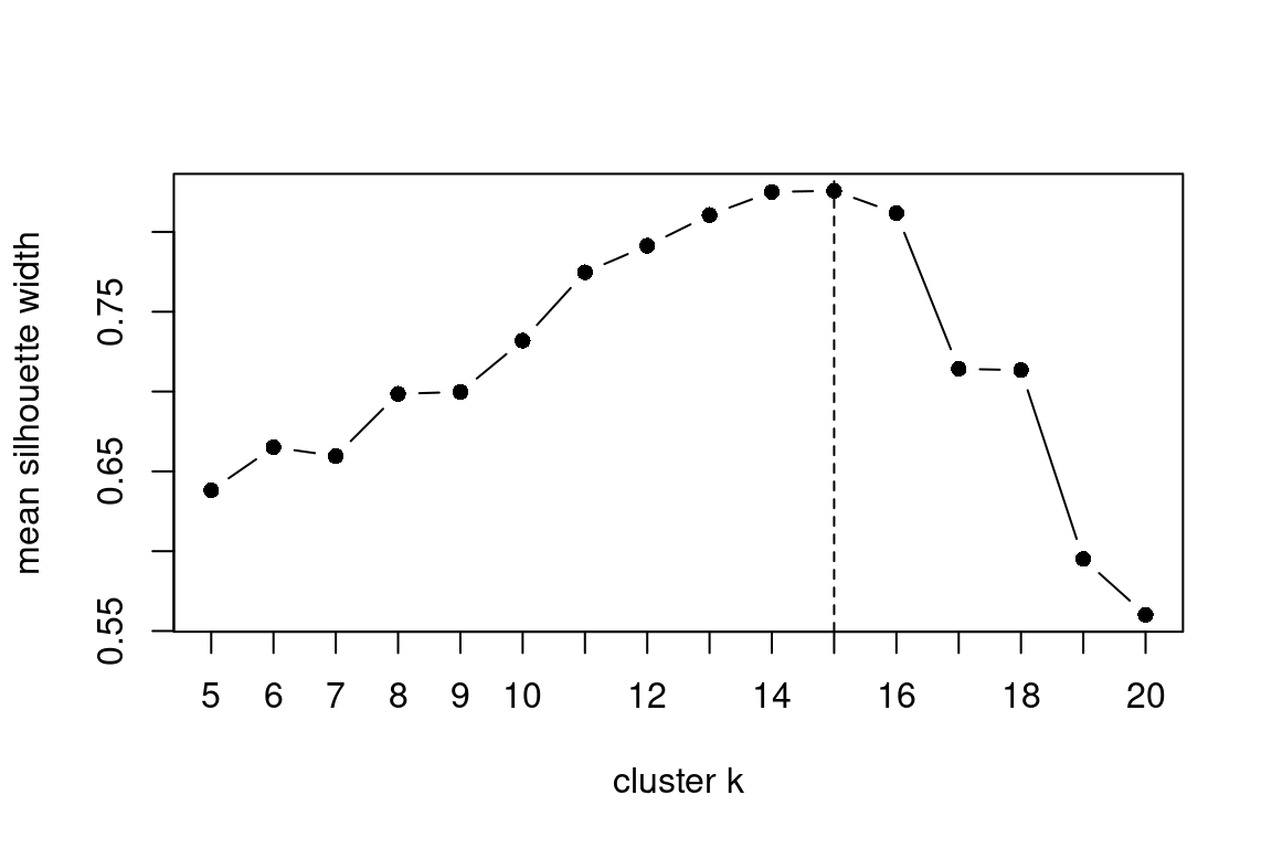
plotSilhouettes() |
componentsClust |
Plot silhouette information to determine the cluster amount |
plotStructure() |
compoundsCluster |
Plots the maximum common substructure (MCS) of a cluster |

5.9.5 Generating EICs in DataAnalysis
If you have Bruker data and the DataAnalysis software installed, you can automatically add EIC data in a DataAnalysis session. The addDAEIC() will do this for a single m/z in one analysis, whereas the addAllDAEICs() function adds EICs for all features in a featureGroups object.
# add a single EIC with background subtraction
addDAEIC("mysample", "~/path/to/sample", mz = 120.1234, bgsubtr = TRUE)
# add TIC for MS/MS signal of precursor 120.1234 (value of mz is ignored for TICs)
addDAEIC("mysample", "~/path/to/sample", mz = 100, ctype = "TIC",
         mtype = "MSMS", fragpath = "120.1234", name = "MSMS 120")

addAllDAEICs(fGroups) # add EICs for all features
addAllDAEICs(fGroups[, 1:50]) # as usual, subsetting can be used for partial data