9.11 Feature regression analysis
Basic support in patRoon is available to perform simple linear regression (using y=ax+b with a the slope b the intercept) on feature intensities vs given x values. The x values typically are experimental conditions such as sampling time or initial concentration of a parent in a degradation experiment. The linearity could then be used as a way to prioritize features (as performed in Helmus et al. (2025)). Originally, this functionality was implemented as a very basic method to perform rough calculations of concentrations. However, the next section describes a much better way by using the MS2Quant package.
The x-values should be specified as metadata in the analysis information, for instance:
# create analysis information: for demonstrative purposes we just base it on the example data
anaInfoRegr <- anaInfo
anaInfoRegr$experiment <- c("UV", "UV", "UV", "H2O2", "H2O2", "H2O2")
anaInfoRegr$exposure <- c(0, 30, 60, 0, 30, 60) # time in minutes
anaInfoRegr[, c("analysis", "experiment", "exposure")]
#> analysis experiment exposure
#> 1 solvent-pos-1 UV 0
#> 2 solvent-pos-2 UV 30
#> 3 solvent-pos-3 UV 60
#> 4 standard-pos-1 H2O2 0
#> 5 standard-pos-2 H2O2 30
#> 6 standard-pos-3 H2O2 60The x-values can be set to NA in case no experimental conditions are available; the regression properties will be calculated from all non-NA data.
The as.data.table() function (or as.data.frame()) can then be used to calculate regression data:
# use areas for regression calculation and make sure that feature data is reported
# the exposure metadata is used as x values, the experiment metadata is used to calculate the regression for analyses groups
# (only relevant columns are shown for clarity)
as.data.table(fGroupsRegr, areas = TRUE, features = TRUE,
              regression = "exposure", regressionBy = "experiment")[, .(analysis, group, x_reg, RSQ, intercept, slope, p)]
#> analysis group x_reg RSQ intercept slope p
#> <char> <char> <num> <num> <num> <num> <num>
#> 1: solvent-pos-1 M99_R14_1 -765.0052 0.99525396 4351423 5176.367 0.04389244
#> 2: solvent-pos-2 M99_R14_1 -775.8074 0.99525396 4351423 5176.367 0.04389244
#> 3: solvent-pos-3 M99_R14_1 -778.7245 0.99525396 4351423 5176.367 0.04389244
#> 4: standard-pos-1 M99_R14_1 710.7070 0.90164426 4814974 -6310.333 0.20308172
#> 5: standard-pos-2 M99_R14_1 716.6610 0.90164426 4814974 -6310.333 0.20308172
#> ---
#> 2922: solvent-pos-2 M433_R10_680 -538.6387 0.99048530 2595803 3329.317 0.06219692
#> 2923: solvent-pos-3 M433_R10_680 -534.8049 0.99048530 2595803 3329.317 0.06219692
#> 2924: standard-pos-1 M433_R10_680 1635.3435 0.06340353 3078297 -1303.883 0.83795459
#> 2925: standard-pos-2 M433_R10_680 1716.0164 0.06340353 3078297 -1303.883 0.83795459
#> 2926: standard-pos-3 M433_R10_680 1660.7139 0.06340353 3078297 -1303.883 0.83795459The regressionBy argument in the above example is set to ensure that regression is calculated for each experiment separately. In sets workflows you can set regressionBy="set" to perform the calculations per set. The regressionBy argument can be omitted if the regression should be calculated for all analyses together. The x_reg output column stores the x values calculated by the regression model (only present if features=TRUE). Other regression properties such as the RSQ, slope and p can be used as a basic trend analysis for prioritization:
fGroupsTab <- as.data.table(fGroupsRegr, areas = TRUE, features = TRUE,
                            regression = "exposure", regressionBy = "experiment")
# subset features that appear to increase in intensity with longer UV exposure
increasingFGroups <- fGroupsRegr[, fGroupsTab[RSQ >= 0.8 & p < 0.05 & slope > 0, group]]
The plotInt() function can also work with regression data and is helpful for visualization purposes.
# plot regression for a specific feature group
plotInt(fGroupsRegr[, 13], areas = TRUE, regression = TRUE, xBy = "exposure",
        groupBy = "experiment", showLegend = TRUE)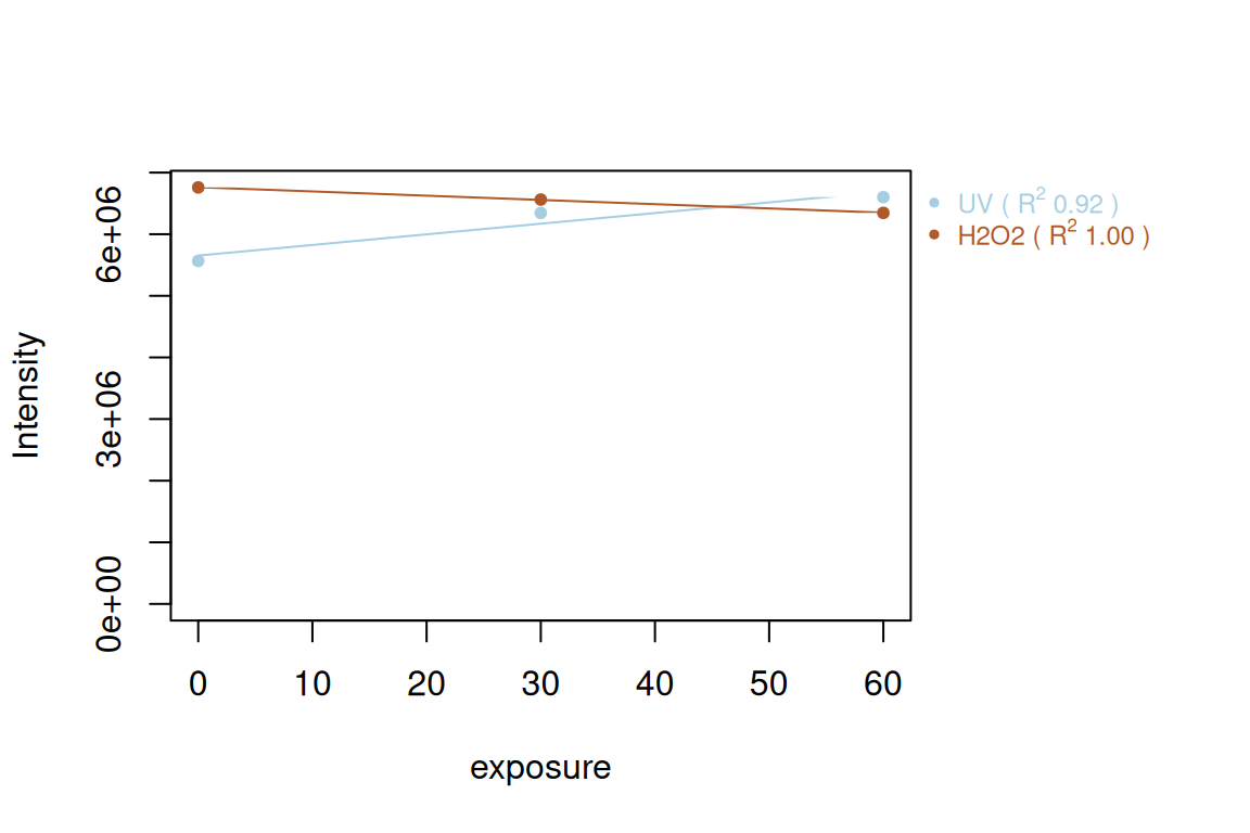
For more details, see the reference manual for the feature groups methods for as.data.table() and plotInt() (?as.data.table and ?plotInt).