9.13 Fold changes
A specific statistical way to prioritize feature data is by Fold changes (FC). This is a relative simple method to quickly identify (significant) changes between two sample groups. A typical use case is to compare the feature intensities before and after an experiment.
To perform FC calculations we first need to specify its parameters. This is best achieved with the getFCParams() function:
#> $replicates
#> [1] "before" "after"
#>
#> $thresholdFC
#> [1] 0.25
#>
#> $thresholdPV
#> [1] 0.05
#>
#> $zeroMethod
#> [1] "add"
#>
#> $zeroValue
#> [1] 0.01
#>
#> $PVTestFunc
#> function (x, y)
#> t.test(x, y, paired = TRUE)$p.value
#> <bytecode: 0x561d74b5ece0>
#> <environment: 0x561d74b5f3a8>
#>
#> $PVAdjFunc
#> function (pv)
#> p.adjust(pv, "BH")
#> <bytecode: 0x561d74b5eff0>
#> <environment: 0x561d74b5f3a8>
In this example we generate a list with parameters in order to make a comparison between two replicates: before and after. Several advanced parameters are available to tweak the calculation process. These are explained in the reference manual (?featureGroups).
The as.data.table function for feature groups is used to perform the FC calculations.
myFCParams <- getFCParams(c("solvent-pos", "standard-pos")) # compare solvent/standard
as.data.table(fGroups, FCParams = myFCParams)[, c("group", "FC", "FC_log", "PV", "PV_log", "classification")]
#> group FC FC_log PV PV_log classification
#> <char> <num> <num> <num> <num> <char>
#> 1: M99_R14_1 8.837494e-01 -0.17829070 0.223506802 0.65070926 insignificant
#> 2: M99_R4_2 8.500464e-01 -0.23438649 0.778488444 0.10874783 insignificant
#> 3: M100_R7_3 8.009186e-01 -0.32027248 0.804751489 0.09433821 FC
#> 4: M100_R5_4 4.140000e+06 21.98119934 0.533213018 0.27309926 FC
#> 5: M100_R28_5 9.594972e-01 -0.05964952 0.975712373 0.01067819 insignificant
#> ---
#> 676: M425_R319_676 2.149907e+07 24.35777069 0.009681742 2.01404652 increase
#> 677: M427_R10_677 1.059937e+00 0.08397893 0.371260940 0.43032074 insignificant
#> 678: M427_R319_678 7.776800e+06 22.89074521 0.533213018 0.27309926 FC
#> 679: M432_R383_679 9.816400e+06 23.22676261 0.347009089 0.45965915 FC
#> 680: M433_R10_680 1.132909e+00 0.18003240 0.293217996 0.53280938 insignificantThe classification column allows you to easily identify if and how a feature changes between the two sample groups. This can also be used to prioritize feature groups:
tab <- as.data.table(fGroups, FCParams = myFCParams)
# only keep feature groups that significantly increase or decrease
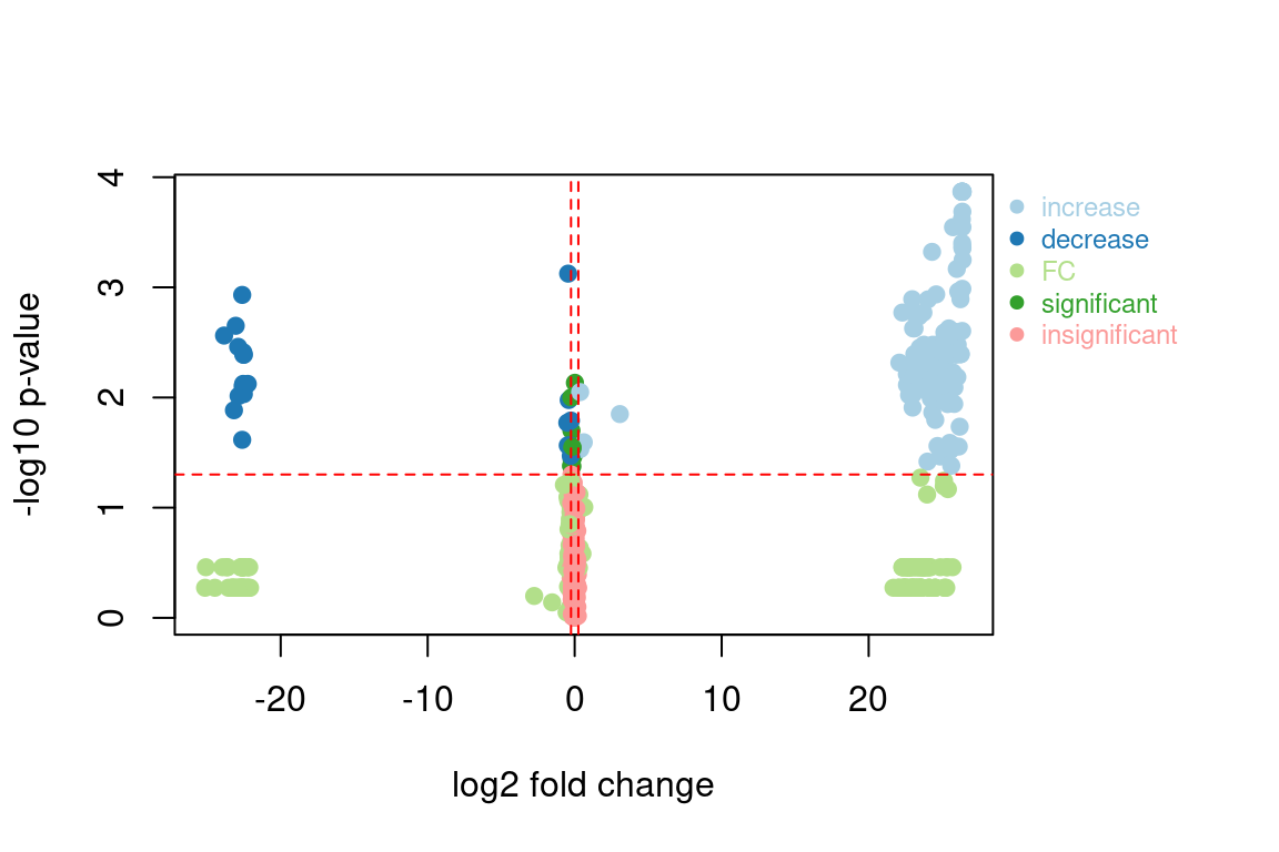
fGroupsChanged <- fGroups[, tab[classification %in% c("increase", "decrease")]$group]The plotVolcano function can be used to visually the FC data: