Introduction
In this tutorial you will learn how to perform a simple non-target
analysis with patRoon. This tutorial is not meant to give a
detailed overview of patRoon. Instead, it serves as a quick
introduction on how to use patRoon to setup and perform a
full non-target analysis workflow.
The workflow in this tutorial consists of the following steps:
Data
In this tutorial we will use example data provided within the patRoonData
package. Please make sure this package is installed (see the Handbook
for brief installation instructions). The example dataset contains LC-MS
data for a standard mixture with known composition (‘standard-X’) and a
blank solvent (‘solvent-X’), both in triplicate and measured with
positive and negative ionization. While this may not seem like the most
exciting data, it does allow to demonstrate the most important
functionality of patRoon.
The provided analyses already have been exported to an open format
(.mzML) and are ready to use. For your own data it may be
necessary to first export your data to mzXML or mzML
and perform other data pre-treatment steps such as mass re-calibration.
This can be done using the tools from ProteoWizard or software
from your mass spectrometer vendor. Alternatively, patRoon
can do this automatically for your analyses with the
convertMSFiles() function. Please see the handbook and
reference manual for its usage.
New project
Whenever you start a new non-target analysis it is highly recommended
to start this from a fresh project directory. This directory
will contain your R processing script(s) and any other
output generated during the workflow. Note that this directory does not
have to contain the raw MS data files. In fact, keeping these files
separate may be handy, for instance, if you want to run multiple
non-target analyses on these files or store the analysis files on a
shared location.
Starting a new project typically consists of
- Creating a new directory (unsurprisingly!)
- Changing the active working directory to the project directory
(e.g. with
setwd()). - Create (or copy) an
Rprocessing script.
Note that step 2 is important as any output files (e.g. reports and
cached results) are stored to the current working directory by default.
Consequently, always take care to ensure that this directory is active,
for instance, after restarting R.
Steps 1-3 can be easily performed with the newProject()
function. Alternatively, you can of course also perform these steps
yourself. Both approaches will be discussed in the next sections.
Automatic project creation
Ensure that RStudio is active and start the new project utility:
patRoon::newProject()NOTE Currently
newProject()only works when using RStudio.
A dialog should pop-up (see screenshot below) where you can specify where and how the new project will be generated, which analyses you want to include and define a basic workflow. Based on this input a new project with a template script will be automatically generated.
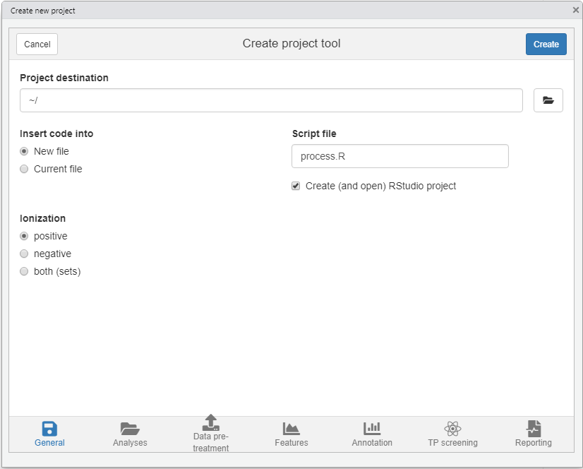
For this tutorial make the following selections
- Destination tab Select your desired location of the new project. Leave other settings as they are.
- Analyses tab Here you normally select your analyses. However, for this tutorial simply select the Example data option.
- Data pre-treatment tab Since the example data is already ready to use you can simply skip this tab.
- Features tab Leave the default OpenMS algorithm for feature finding and grouping.
- Annotation tab Select GenForm and MetFrag for the formula and compound annotation algorithms, respectively.
- TP screening tab No need to do anything here for this tutorial.
- Reporting tab Make sure to enable HTML reporting.
Manual project creation
For RStudio users it is easiest to simply create a new RStudio project (e.g. File –> New Project). This will create a new directory and ensure that the working directory is set whenever you re-open it. Alternatively, you can do this manually, for instance:
projDir <- "~/myProjectDir"
dir.create(projDir)
setwd(projDir)
The next step is to create a new R script. For this
tutorial simply copy the script that is shown in the next section to a
new .R file.
Template R script
After you ran newProject() the file below will be
created. Before running this script, however, we still have to add and
modify some of its code. In the next sections you will learn more about
each part of the script, make the necessary changes and run its
code.
# Script automatically generated on Tue Feb 17 08:05:32 2026

library(patRoon)

# -------------------------
# initialization
# -------------------------

workPath <- "C:/myproject"
setwd(workPath)

# Example data from patRoonData package (triplicate solvent blank + triplicate standard)
anaInfo <- patRoonData::exampleAnalysisInfo("positive")

# -------------------------
# features
# -------------------------

# Find all features
# NOTE: see the reference manual for many more options
fList <- findFeatures(anaInfo, "openms", noiseThrInt = 1000, chromSNR = 3, chromFWHM = 5, minFWHM = 1, maxFWHM = 30)

# Group and align features between analyses
fGroups <- groupFeatures(fList, "openms", rtalign = TRUE)

# Basic rule based filtering
fGroups <- filter(fGroups, preAbsMinIntensity = 100, absMinIntensity = 10000, relMinReplicateAbundance = 1,
                  maxReplicateIntRSD = 0.75, blankThreshold = 5, removeBlanks = TRUE, retentionRange = NULL,
                  mzRange = NULL)

# Update group properties
fGroups <- updateGroups(fGroups, what = c("ret", "mz", "mobility"), intWeight = FALSE)

# -------------------------
# annotation
# -------------------------

# Retrieve MS peak lists
avgMSListParams <- getDefAvgPListParams(clusterMzWindow = 0.005)
mslists <- generateMSPeakLists(fGroups, avgFeatParams = avgMSListParams, avgFGroupParams = avgMSListParams)
# Rule based filtering of MS peak lists. You may want to tweak this. See the manual for more information.
mslists <- filter(mslists, MSLevel = 2, absMinIntensity = NULL, relMinIntensity = 0.05, topMostPeaks = 25,
                  maxMZOverPrec = 4)

# Calculate formula candidates
formulas <- generateFormulas(fGroups, mslists, "genform", adduct = "[M+H]+", elements = "CHNOP", oc = FALSE,
                             calculateFeatures = FALSE)
formulas <- estimateIDConfidence(formulas, IDFile = "idlevelrules.yml")

# Calculate compound structure candidates
compounds <- generateCompounds(fGroups, mslists, "metfrag", adduct = "[M+H]+", database = "pubchemlite",
                               maxCandidatesToStop = 2500)
compounds <- addFormulaScoring(compounds, formulas, updateScore = TRUE)

compounds <- estimateIDConfidence(compounds, MSPeakLists = mslists, formulas = formulas, IDFile = "idlevelrules.yml")

# -------------------------
# reporting
# -------------------------

# Advanced report settings can be edited in the report.yml file.
report(fGroups, MSPeakLists = mslists, formulas = formulas, compounds = compounds, components = NULL,
       settingsFile = "report.yml", openReport = TRUE)
Workflow
Now that you have generated a new project with a template script it is time to make some minor modifications and run it afterwards. In the next sections each major part of the script (initialization, finding and grouping features, annotation and reporting) will be discussed separately. Each section will briefly discuss the code, what needs to be modified and finally you will run the code. In addition, several functions will be demonstrated that you can use to inspect generated data.
Initialization
The first part of the script loads patRoon, makes sure
the current working directory is set correctly and loads information
about the analyses. This part in your script looks more or less like
this:
library(patRoon)

workPath <- "C:/my_project"
setwd(workPath)

# Example data from patRoonData package (triplicate solvent blank + triplicate standard)
anaInfo <- patRoonData::exampleAnalysisInfo("positive")
After you ran this part the analysis information should be stored in
the anaInfo variable. This information is important as it
will be required for subsequent steps in the workflow. Lets peek at its
contents:
anaInfo#> analysis path_centroid path_raw path_profile path_ims replicate blank
#> 1 solvent-pos-1 /usr/local/lib/R/site-library/patRoonData/extdata/pos solvent-pos solvent-pos
#> 2 solvent-pos-2 /usr/local/lib/R/site-library/patRoonData/extdata/pos solvent-pos solvent-pos
#> 3 solvent-pos-3 /usr/local/lib/R/site-library/patRoonData/extdata/pos solvent-pos solvent-pos
#> 4 standard-pos-1 /usr/local/lib/R/site-library/patRoonData/extdata/pos standard-pos solvent-pos
#> 5 standard-pos-2 /usr/local/lib/R/site-library/patRoonData/extdata/pos standard-pos solvent-pos
#> 6 standard-pos-3 /usr/local/lib/R/site-library/patRoonData/extdata/pos standard-pos solvent-posAs you can see the generated data.frame consists of the
following columns:
-
path_*: columns that specify the directory paths to the
analysis files, in raw, centroided, profile and ims format. The
path_centroidcolumn is only used in most workflows. - analysis: the name of the analysis. This should be the file name without file extension.
- replicate: to which replicate the analysis belongs. All analysis which are replicates of each other get the same name.
- blank: which replicate should be used for blank subtraction.
The latter two columns are especially important for data cleanup, which will be discussed later.
For now keep in mind that the analyses for the solvents and standards
each belong to a different replicate ("solvent" and
"standard") and that the solvents should be used for blank
subtraction.
In this tutorial the analysis information was just copied directly
from patRoonData. The
generateAnalysisInfo() function can be used to generate
such a table for your own sample analyses. This function scans a given
directory for MS data files and automatically fills in the
path and analysis columns from this
information. In addition, you can pass replicate and blank information
to this function. Example:
generateAnalysisInfo(fromCentroid = patRoonData::exampleDataPath(), replicate = c(rep("solvent-pos", 3), rep("standard-pos", 3)),
                     blank = "solvent")
#> analysis path_centroid path_raw path_profile path_ims replicate blank
#> 1 solvent-pos-1 /usr/local/lib/R/site-library/patRoonData/extdata/pos solvent-pos solvent
#> 2 solvent-pos-2 /usr/local/lib/R/site-library/patRoonData/extdata/pos solvent-pos solvent
#> 3 solvent-pos-3 /usr/local/lib/R/site-library/patRoonData/extdata/pos solvent-pos solvent
#> 4 standard-pos-1 /usr/local/lib/R/site-library/patRoonData/extdata/pos standard-pos solvent
#> 5 standard-pos-2 /usr/local/lib/R/site-library/patRoonData/extdata/pos standard-pos solvent
#> 6 standard-pos-3 /usr/local/lib/R/site-library/patRoonData/extdata/pos standard-pos solventNOTE Of course nothing stops you from creating a
data.framewith analysis information manually withinRor load the information from a csv file. In fact, when you create a new project withnewProject()you can select to generate a separate csv file with analysis information (i.e. by filling in the right information in the analysis tab).
NOTE The blanks for the solvent analyses are set to themselves. This will remove any features from the solvents later in the workflow, which is generally fine as we are usually not interested in the blanks anyway.
Find and group features
The first step of a LC-MS non-target analysis workflow is typically the extraction of so called ‘features’. While sometimes slightly different definitions are used, a feature can be seen as a single peak within an extracted ion chromatogram. For a complex sample it is not uncommon that hundreds to thousands of features can extracted. Because these large numbers this process is typically automatized nowadays.
To obtain all the features within your dataset the
findFeatures function is used. This function requires data
on the analysis information (anaInfo variable created
earlier) and the desired algorithm that should be used. On top of that
there are many more options that can significantly influence the feature
finding process, hence, it is important to evaluate results
afterwards.
In this tutorial we will use the OpenMS software to find features and stick with default parameters:
fList <- findFeatures(anaInfo, "openms", noiseThrInt = 1000, chromSNR = 3, chromFWHM = 5, minFWHM = 1, maxFWHM = 30)#> Finding features with OpenMS for 6 analyses ...
#> ================================================================================
#> Loading peak intensities...
#> Using 'mzr' backend for reading MS data.
#> ================================================================================
#> Done!
#> Feature statistics:
#> solvent-pos-1: 3760 (15.4%)
#> solvent-pos-2: 3719 (15.3%)
#> solvent-pos-3: 3820 (15.7%)
#> standard-pos-1: 4373 (17.9%)
#> standard-pos-2: 4486 (18.4%)
#> standard-pos-3: 4222 (17.3%)
#> Total: 24380After some processing time (especially for larger datasets), the next step is to group features. During this step, features from different analysis are grouped, optionally after alignment of their retention times. This grouping is necessary because it is common that instrumental errors will result in (slight) variations in both retention time and m/z values which may complicate comparison of features between analyses. The resulting groups are referred to as feature groups and are crucial input for subsequent workflow steps.
To group features the groupFeatures() function is
used:
fGroups <- groupFeatures(fList, "openms", rtalign = TRUE)#> Grouping features with OpenMS...
#> ===========
#> Importing consensus XML...Done!
#>
#> ===========
#> Done!The Handbook
and reference manual (?findFeatures and
?groupFeatures) lists many more algorithms and parameters
that can be used for both feature finding and grouping.
Data clean-up
The next step is to perform some basic rule based filtering with the
filter() function. As its name suggests this function has several ways
to filter data. It is a so called generic function and methods exists
for various data types, such as the feature groups object that was made
in the previous section (stored in the the fGroups
variable). Note that in this tutorial the absMinIntensity
was increased to 1E5 to simplify the results.
fGroups <- filter(fGroups, preAbsMinIntensity = 100, absMinIntensity = 1E5,
                  relMinReplicateAbundance = 1, maxReplicateIntRSD = 0.75,
                  blankThreshold = 5, removeBlanks = TRUE,
                  retentionRange = NULL, mzRange = NULL)
#> Applying intensity filter... Done! Filtered 0 (0.00%) features and 0 (0.00%) feature groups. Remaining: 24380 features in 7302 groups.
#> Applying replicate abundance filter... Done! Filtered 8006 (32.84%) features and 3849 (52.71%) feature groups. Remaining: 16374 features in 3453 groups.
#> Applying blank filter... Done! Filtered 13558 (82.80%) features and 2514 (72.81%) feature groups. Remaining: 2816 features in 939 groups.
#> Applying intensity filter... Done! Filtered 2429 (86.26%) features and 806 (85.84%) feature groups. Remaining: 387 features in 133 groups.
#> Applying replicate abundance filter... Done! Filtered 15 (3.88%) features and 9 (6.77%) feature groups. Remaining: 372 features in 124 groups.
#> Applying replicate filter... Done! Filtered 0 (0.00%) features and 0 (0.00%) feature groups. Remaining: 372 features in 124 groups.The following filtering steps will be performed:
- Features are removed if their intensity is below a defined intensity
threshold (set by
absMinIntensity). This filter is an effective way to not only remove ‘noisy’ data, but, for instance, can also be used to remove any low intensity features which likely miss MS/MS data. - If a feature is not ubiquitously present in (part of) replicate
analyses it will be filtered out from that replicate. This is controlled
by setting
relMinReplicateAbundance. The value is relative, for instance, a value of0.5would mean that a feature needs to be present in half of the replicates. In this tutorial we use a value of1which means that a feature should be present in all replicate samples. This is a very effective filter in removing any false positives, for instance, caused by features which don’t actually represent a well defined chromatographic peak. - Similarly, the features within a replicate are removed if the
relative standard deviation (RSD) of their intensities exceeds that of
the value set by the
maxReplicateIntRSDargument. - Features are filtered out that do not have a significantly higher
intensity than the blank intensity. This is controlled by
blankThreshold: the given value of5means that the intensity of a feature needs to be at least five times higher compared to the (average) blank signal.
The removeBlanks argument tells will remove all blank
analyses after filtering. The retentionRange and
mzRange arguments are not used here, but could be used to
filter out any features outside a give retention or m/z range.
There are many more filters: see ?filter() for more
information.
As you may have noticed quite a large part of the features are removed as a result of the filtering step. However, using the right settings is a very effective way to separate interesting data from the rest.
The next logical step in a non-target workflow is often to perform further prioritization of data. However, this will not be necessary in this tutorial as our samples are just known standard mixtures.
After cleaning up the data, the updateGroups() function
is called to update the feature group properties (retention time and
m/z). This can improve their accuracy, since e.g. false positives don’t
attribute to the group properties anymore.
fGroups <- updateGroups(fGroups, what = c("ret", "mz", "mobility"), intWeight = FALSE)To simplify processing, we only continue with the first 25 feature groups:
fGroups <- fGroups[, 1:25]Inspecting results
In order to have a quick peek at the results we can use the default printing method:
fGroups#> A featureGroupsOpenMS object
#> Hierarchy:
#> featureGroups
#> |-- featureGroupsOpenMS
#> ---
#> Object size (indication): 56.6 kB
#> Algorithm: openms
#> Feature groups: M100_R28_65, M102_R7_94, M109_R192_157, M116_R316_229, M120_R268_288, M134_R301_482, ... (25 total)
#> Features: 75 (3.0 per group)
#> Has IMS data: no
#> Has normalized intensities: FALSE
#> Internal standards used for normalization: no
#> Predicted concentrations: none
#> Predicted toxicities: none
#> Analyses: standard-pos-1, standard-pos-2, standard-pos-3 (3 total)
#> Replicates: standard-pos (1 total)
#> Replicates used as blank: solvent-pos (1 total)Furthermore, the as.data.table() function can be used to
have a look at generated feature groups and their intensities
(i.e. peak heights) across all analyses:
as.data.table(fGroups)#> group ret mz standard-pos-1_intensity standard-pos-2_intensity standard-pos-3_intensity
#> <char> <num> <num> <num> <num> <num>
#> 1: M100_R28_65 27.77433 100.1120 304644 275468 283104
#> 2: M102_R7_94 7.12500 102.1277 342224 320876 327020
#> 3: M109_R192_157 191.79933 109.0759 186612 187080 176756
#> 4: M116_R316_229 316.04800 116.0527 742572 772332 851204
#> 5: M120_R268_288 268.36133 120.0554 264836 245372 216560
#> ---
#> 21: M171_R226_1209 226.30333 171.0648 190596 171880 155088
#> 22: M180_R336_1410 335.51633 180.0804 143896 156384 135340
#> 23: M183_R193_1487 192.96133 183.0627 274544 250108 234716
#> 24: M183_R313_1489 312.67033 183.0779 682396 849328 665428
#> 25: M186_R293_1568 292.47467 186.2213 487912 488284 509880An overview of group properties is returned by the
groupInfo() method:
#>            group       ret       mz
#>           <char>     <num>    <num>
#> 1:   M100_R28_65  27.77433 100.1120
#> 2:    M102_R7_94   7.12500 102.1277
#> 3: M109_R192_157 191.79933 109.0759
#> 4: M116_R316_229 316.04800 116.0527
#> 5: M120_R268_288 268.36133 120.0554
#> 6: M134_R301_482 301.28933 134.0710
Finally, we can have a quick look at our data by plotting some nice extracted ion chromatograms (EICs) for all feature groups:
plotChroms(fGroups, groupBy = "fGroups", showFGroupRect = FALSE, showPeakArea = TRUE,
           EICParams = getDefEICParams(topMost = 1), showLegend = FALSE)
#> Using 'mzr' backend for reading MS data.
#> ================================================================================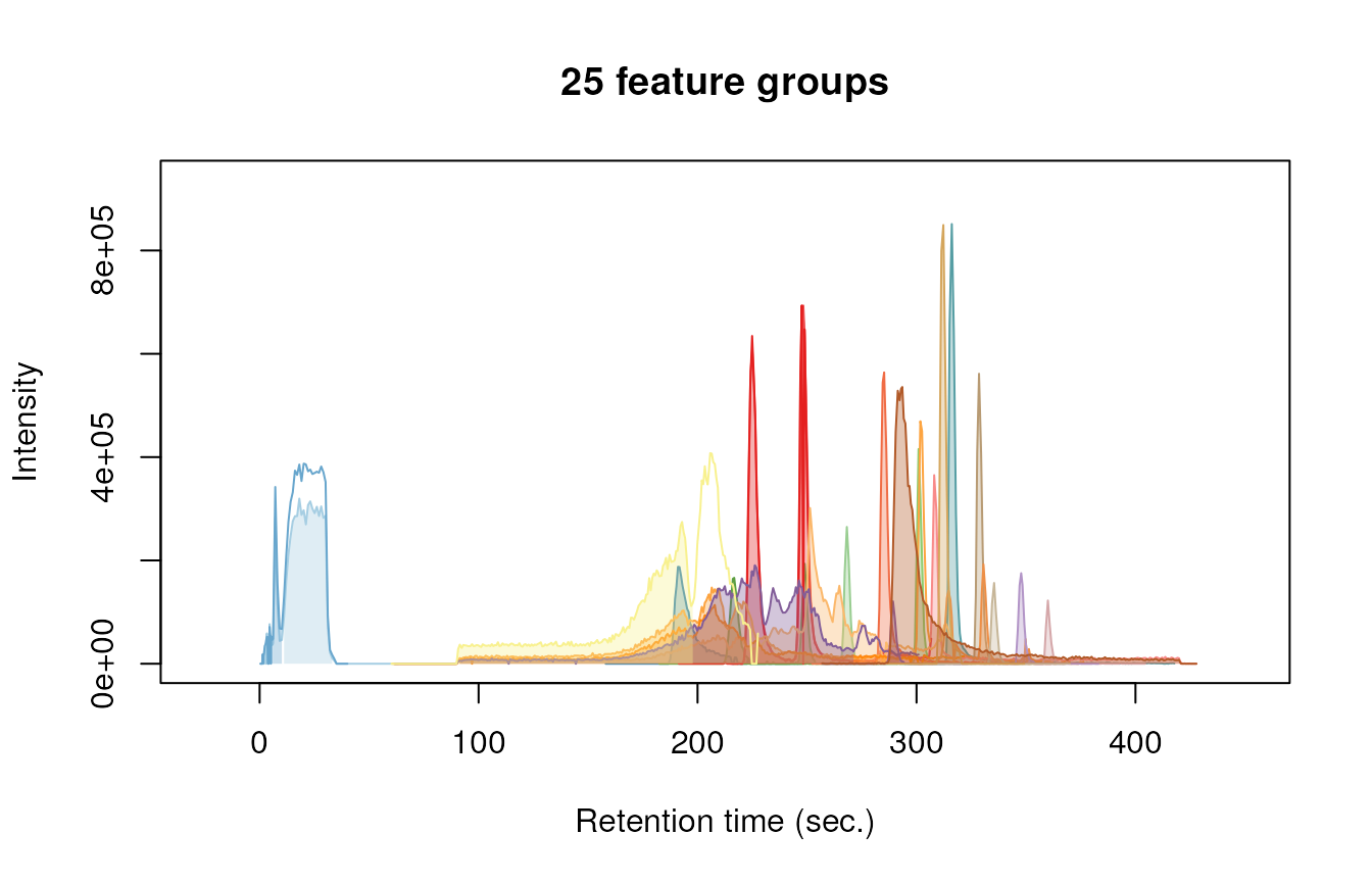
Note that we only plot the most intense feature of a feature group
here (as set by topMost=1). See the reference docs for many
more parameters to these functions (e.g. ?plotChroms).
Annotation
MS peak lists
After obtaining a good dataset with features of interest we can start moving to find their chemical identity. Before doing so, however, the first step is to extract all relevant MS data that will be used for annotation. The tutorial data was obtained with data-dependent MS/MS, so in the ideal case we can obtain both MS and MS/MS data for each feature group.
The generateMSPeakLists() function will perform this
action for us and will generate so called MS peak lists in the
process. These lists are basically (averaged) spectra in a tabular
form.
avgPListParams <- getDefAvgPListParams(clusterMzWindow = 0.002)
mslists <- generateMSPeakLists(fGroups, avgFeatParams = avgPListParams, avgFGroupParams = avgPListParams)#> Loading all MS peak lists for 25 feature groups and 3 analyses...
#> Using 'mzr' backend for reading MS data.
#> ================================================================================
#> Generating averaged peak lists for all feature groups... Done!Note that we lowered the clusterMzWindow value to
0.002. This window is used during averaging to cluster similar
m/z values together. In general the better the resolution of
your MS instrument, the lower the value can be set.
Similar to feature groups the filter() generic function
can be used to clean up the peak lists afterwards:
mslists <- filter(mslists, MSLevel = 2, absMinIntensity = NULL, relMinIntensity = 0.02, topMostPeaks = 10,
                  maxMZOverPrec = 4)
#> Done! Filtered 1332 (15.42%) MS peaks. Remaining: 7307This step removes all MS/MS peaks that are
- below 2% of the most intense peak in the spectrum (as set by
relMinIntensity). - more than 4 m/z units above the precursor m/z (as
set by
maxMZOverPrec). - From the remaining peaks, no more than the ten most intense peaks
are retained (as set by
topMostPeaks).
Formula annotation
Using the data from the MS peak lists generated during the previous step we can generate a list of formula candidates for each feature group which is based on measured m/z values, isotopic patterns and presence of MS/MS fragments. In this tutorial we will use this data as an extra hint to score candidate chemical structures generated during the next step. The code below will use GenForm to perform this step. Again running this code may take some time.
formulas <- generateFormulas(fGroups, mslists, "genform", adduct = "[M+H]+", elements = "CHNOPSCl",
                             oc = FALSE, calculateFeatures = FALSE)
#> Loading all formulas...
#> Converting to algorithm specific adducts... Done!
#> ================================================================================
#> Loaded 36 formulas for 23 feature groups (92.00%).
#> Calculating annotation similarities... Done!
formulas <- estimateIDConfidence(formulas, IDFile = "idlevelrules.yml")#> Estimating identification levels for 23 feature groups with a total of 36 candidates...#> ================================================================================Note that you may need to change the elements parameter to this
function, e.g. here to make sure that formulae with sulfur and chloride
(S/Cl) are also calculated. It is highly recommended to limit the
elements (by default it is just C, H, N, O and P) as this can
significantly reduce processing time and improbable formula candidates.
In this tutorial we already knew which compounds to expect so the choice
was easy, but often a good guess can be made in advance. The call the
estimateIDConfidence() function is then used to estimate
the confidence of the generated formula candidates based on a set of
rules defined in the idlevelrules.yml file. This file is
based on the Schymanski ID
confidence levels and can be modified to fit your needs.
Compound annotation
Now it is time to actually see what compounds we may be dealing with.
In this tutorial we will use MetFrag to come up with a
list of possible candidate structures for each feature group. Before we
can start you have to make sure that MetFrag and the PubChemLite library
can be found by patRoon. Please see the Handbook
for installation instructions.
Then generateCompounds() is used to execute MetFrag and
generate the compounds.
compounds <- generateCompounds(fGroups, mslists, "metfrag", adduct = "[M+H]+", database = "pubchemlite",
                               maxCandidatesToStop = 2500)
#> Identifying 25 feature groups with MetFrag...
#> Converting to algorithm specific adducts... Done!
#> ================================================================================
#> Loaded 936 compounds from 19 features (76.00%).
#> Calculating annotation similarities... Done!See ?generateCompounds() for more information on
possible databases and many other parameters that can be set.
NOTE This is often one of the most time consuming steps during the workflow. For this reason you should always take care to prioritize your data before running this function!
Finally we use the addFormulaScoring() function to
improve ranking of candidates by incorporating the formula calculation
data from the previous step, and use estimateIDConfidence()
again to estimate identification confidence levels for each of the
candidates.
compounds <- addFormulaScoring(compounds, formulas, updateScore = TRUE)#> Adding formula scoring...
#> ================================================================================
compounds <- estimateIDConfidence(compounds, MSPeakLists = mslists, formulas = formulas, IDFile = "idlevelrules.yml")#> Estimating identification levels for 19 feature groups with a total of 936 candidates...
#> ================================================================================Inspecting results
Similar as feature groups we can quickly peek at some results:
mslists#> A MSPeakLists object
#> Hierarchy:
#> workflowStep
#> |-- MSPeakLists
#> |-- MSPeakListsSet
#> |-- MSPeakListsUnset
#> ---
#> Object size (indication): 844.6 kB
#> Algorithm: patroon
#> Total peak count: 7307 (MS: 6860 - MS/MS: 447)
#> Average peak count/analysis: 2436 (MS: 2287 - MS/MS: 149)
#> Total peak lists: 128 (MS: 75 - MS/MS: 53)
#> Average peak lists/analysis: 43 (MS: 25 - MS/MS: 18)
formulas#> A formulas object
#> Hierarchy:
#> featureAnnotations
#> |-- formulas
#> |-- formulasConsensus
#> |-- formulasSet
#> |-- formulasConsensusSet
#> |-- formulasUnset
#> |-- formulasSIRIUS
#> ---
#> Object size (indication): 216.4 kB
#> Algorithm: genform
#> Formulas assigned to features:
#> - Total formula count: 0
#> - Average formulas per analysis: 0.0
#> - Average formulas per feature: 0.0
#> Formulas assigned to feature groups:
#> - Total formula count: 36
#> - Average formulas per feature group: 1.6
compounds#> A compoundsMF object
#> Hierarchy:
#> compounds
#> |-- compoundsMF
#> ---
#> Object size (indication): 3.7 MB
#> Algorithm: metfrag
#> Number of feature groups with compounds in this object: 19
#> Number of compounds: 936 (total), 49.3 (mean), 1 - 100 (min - max)
as.data.table(mslists)#> group type ID mz intensity fgroup_abundance_rel fgroup_abundance_abs feat_abundance_rel feat_abundance_abs precursor
#> <char> <char> <int> <num> <num> <num> <num> <num> <num> <lgcl>
#> 1: M100_R28_65 MS 1 97.06464 32521.98 1 3 0.8952991 11.333333 FALSE
#> 2: M100_R28_65 MS 2 98.97523 148481.36 1 3 1.0000000 12.666667 FALSE
#> 3: M100_R28_65 MS 3 100.11201 210341.30 1 3 1.0000000 12.666667 TRUE
#> 4: M100_R28_65 MS 4 101.05956 28012.87 1 3 0.9743590 12.333333 FALSE
#> 5: M100_R28_65 MS 5 102.12772 274810.00 1 3 1.0000000 12.666667 FALSE
#> ---
#> 1511: M186_R293_1568 MSMS 29 125.09600 47036.71 1 3 1.0000000 4.666667 FALSE
#> 1512: M186_R293_1568 MSMS 37 142.15886 59948.36 1 3 1.0000000 4.666667 FALSE
#> 1513: M186_R293_1568 MSMS 39 144.17458 100887.25 1 3 1.0000000 4.666667 FALSE
#> 1514: M186_R293_1568 MSMS 47 186.22173 277026.44 1 3 1.0000000 4.666667 TRUE
#> 1515: M186_R293_1568 MSMS 48 187.22490 42499.82 1 3 1.0000000 4.666667 FALSE
as.data.table(formulas)[, 1:7] # only show first columns for clarity#> group neutral_formula ion_formula neutralMass ion_formula_mz error dbe
#> <char> <char> <char> <num> <num> <num> <num>
#> 1: M100_R28_65 C6H13N C6H14N 99.1048 100.1121 0.7 1
#> 2: M102_R7_94 C6H15N C6H16N 101.1204 102.1277 0.2 0
#> 3: M109_R192_157 C6H8N2 C6H9N2 108.0687 109.0760 0.3 4
#> 4: M116_R316_229 C5H9NS C5H10NS 115.0456 116.0529 1.0 2
#> 5: M120_R268_288 C6H5N3 C6H6N3 119.0483 120.0556 1.6 6
#> ---
#> 32: M183_R193_1487 C5H6N6O2 C5H7N6O2 182.0552 183.0625 -1.7 6
#> 33: M183_R313_1489 C7H15ClO3 C7H16ClO3 182.0710 183.0782 2.1 0
#> 34: M183_R313_1489 C6H15O4P C6H16O4P 182.0708 183.0781 1.1 0
#> 35: M183_R313_1489 CH10N8OS CH11N8OS 182.0698 183.0771 -4.2 1
#> 36: M186_R293_1568 C12H27N C12H28N 185.2143 186.2216 1.3 0
as.data.table(compounds)[, 1:5] # only show first columns for clarity#> group explainedPeaks score neutralMass SMILES
#> <char> <int> <num> <num> <char>
#> 1: M109_R192_157 1 4.166634 108.0687 C1=CC=C(C=C1)NN
#> 2: M109_R192_157 1 3.913405 108.0687 C1=CC(=CC=C1N)N
#> 3: M109_R192_157 1 3.857652 108.0687 C1=CC=C(C(=C1)N)N
#> 4: M109_R192_157 1 3.533509 108.0687 C1=CC(=CC(=C1)N)N
#> 5: M109_R192_157 1 2.895269 108.0687 CC1=CN=C(C=N1)C
#> ---
#> 932: M186_R293_1568 3 2.168060 185.2143 CCCCCCC(CCCC)CN
#> 933: M186_R293_1568 3 2.052083 185.2143 CCCC(CCC)(CC(C)C)NC
#> 934: M186_R293_1568 3 2.052069 185.2143 CCCC(CCC)(CCC)NCC
#> 935: M186_R293_1568 3 2.043274 185.2143 CC(C)CC(C)NC(C)CC(C)C
#> 936: M186_R293_1568 3 2.042262 185.2143 CCCC(CCC)(CCC)N(C)C
plotSpectrum(mslists, "M186_R293_1568", MSLevel = 2)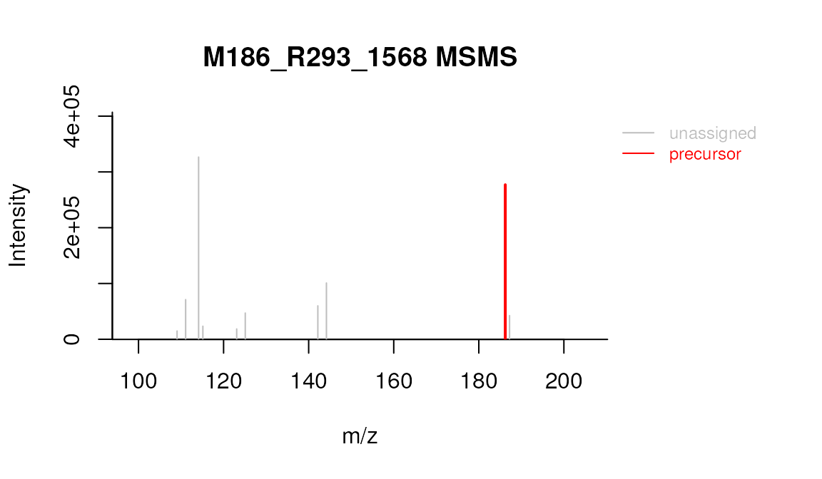
plotSpectrum(formulas, 1, "M109_R192_157", MSPeakLists = mslists)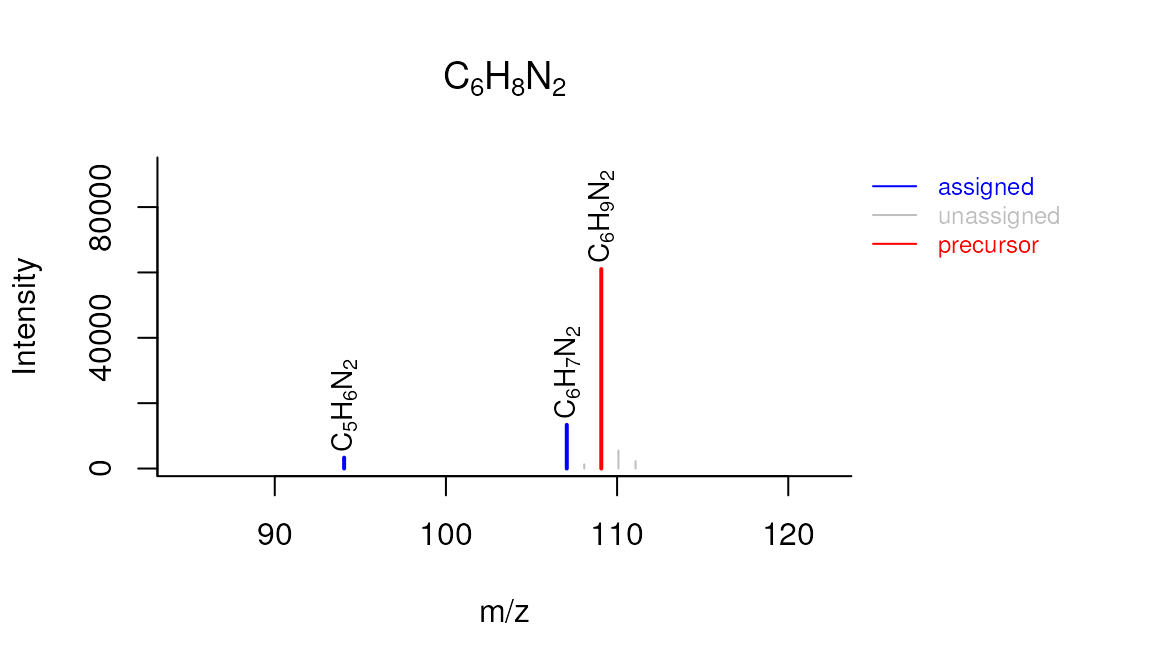
plotSpectrum(compounds, 1, "M120_R268_288", mslists, plotStruct = TRUE)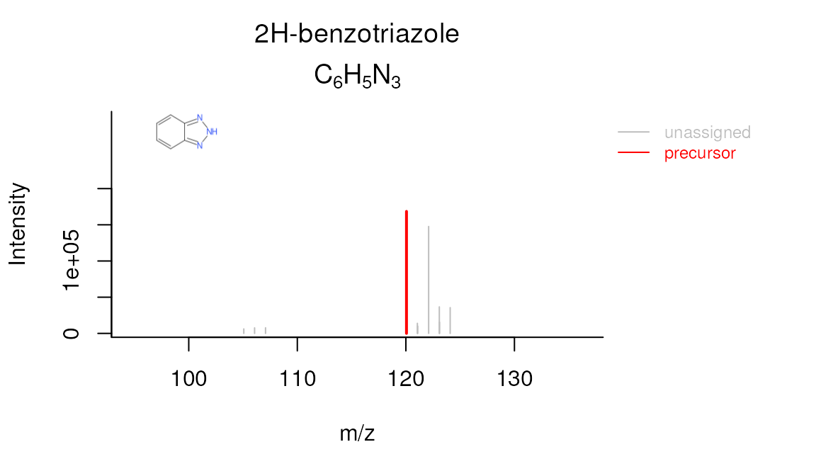
Reporting
The last step of the workflow is typically to report all the data.
The report() function combines all workflow data in an easy
to use interactive HTML document.
report(fGroups, MSPeakLists = mslists, formulas = formulas, compounds = compounds,
       components = NULL, settingsFile = "report.yml", openReport = TRUE)
NOTE If you did not use
newProject()and created the project manually then you first need to generate a new report settings file:
genReportSettingsFile() # only run this if the project was created manually without newProject() The output of report() can be viewed here.
Note that these functions can be called at any time during the workflow. This may be especially useful if you want evaluate results during optimization or exploring the various algorithms and their parameters. In this case you can simply cherry pick the data that you want to report, for instance:
Final script
In the previous sections the different parts of the processing script were discussed and where necessary modified. As a reference, the final script look similar ot this:
# Script automatically generated on Tue Feb 17 08:05:32 2026

library(patRoon)

# -------------------------
# initialization
# -------------------------

workPath <- "C:/myproject"
setwd(workPath)

# Example data from patRoonData package (triplicate solvent blank + triplicate standard)
anaInfo <- patRoonData::exampleAnalysisInfo("positive")

# -------------------------
# features
# -------------------------

# Find all features
# NOTE: see the reference manual for many more options
fList <- findFeatures(anaInfo, "openms", noiseThrInt = 1000, chromSNR = 3, chromFWHM = 5, minFWHM = 1, maxFWHM = 30)

# Group and align features between analyses
fGroups <- groupFeatures(fList, "openms", rtalign = TRUE)

# Basic rule based filtering
fGroups <- filter(fGroups, preAbsMinIntensity = 100, absMinIntensity = 1E5, relMinReplicateAbundance = 1,
                  maxReplicateIntRSD = 0.75, blankThreshold = 5, removeBlanks = TRUE, retentionRange = NULL,
                  mzRange = NULL)

# Update group properties
fGroups <- updateGroups(fGroups, what = c("ret", "mz", "mobility"), intWeight = FALSE)

# -------------------------
# annotation
# -------------------------

# Retrieve MS peak lists
avgMSListParams <- getDefAvgPListParams(clusterMzWindow = 0.002)
mslists <- generateMSPeakLists(fGroups, avgFeatParams = avgMSListParams, avgFGroupParams = avgMSListParams)
# Rule based filtering of MS peak lists. You may want to tweak this. See the manual for more information.
mslists <- filter(mslists, MSLevel = 2, absMinIntensity = NULL, relMinIntensity = 0.02, topMostPeaks = 10,
                  maxMZOverPrec = 4)

# Calculate formula candidates
formulas <- generateFormulas(fGroups, mslists, "genform", adduct = "[M+H]+", elements = "CHNOPSCl", oc = FALSE,
                             calculateFeatures = FALSE)
formulas <- estimateIDConfidence(formulas, IDFile = "idlevelrules.yml")

# Calculate compound structure candidates
compounds <- generateCompounds(fGroups, mslists, "metfrag", adduct = "[M+H]+", database = "pubchemlite",
                               maxCandidatesToStop = 2500)
compounds <- addFormulaScoring(compounds, formulas, updateScore = TRUE)

compounds <- estimateIDConfidence(compounds, MSPeakLists = mslists, formulas = formulas, IDFile = "idlevelrules.yml")

# -------------------------
# reporting
# -------------------------

# Advanced report settings can be edited in the report.yml file.
report(fGroups, MSPeakLists = mslists, formulas = formulas, compounds = compounds, components = NULL,
       settingsFile = "report.yml", openReport = TRUE)